20.1. P-system

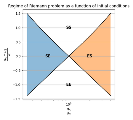
Riemann problem in the P-sys. 1-dimensional P-sys is a two-variable hyperbolic system. Riemann problem for the P-sys aims at finding the two waves (either shock or expansion waves), connecting the uniform regions with conservative variables \(\mathbf{u}_L\), \(\mathbf{u}_R\) on the left and the right of the discontinuity respectively, through one intermediate state \(\mathbf{u}_1\) to be determined as a part of the solution of the Riemann problem.

Numerical solution of a Riemann problem for P-sys

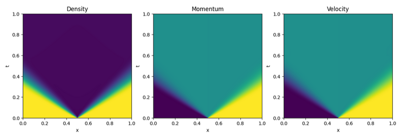
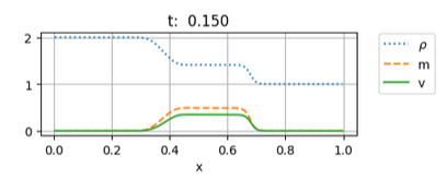
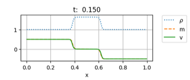
Here, the numerical solution evaluated with a 1-dimensional finite volume solver, using Roe flux with entropy fix (so far, only low-order flux here, withouth high-order…: the solution is affected by numerical dissipation introduced by the Roe flux, essentially an upwind scheme exploiting the characteristic structure of the system and introducing numerical dissipation…). The speed of sound is set as \(a = 1.\)

todo Discuss the solutions, in terms of velocity of the rarefaction and shock waves, using characteristic method and spectral decomposition of the advection matrix

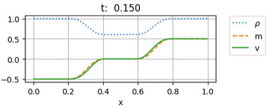
Expansion-expansion. \((\rho_A, u_A) = (1, -.5)\), \((\rho_B, u_B) = (1, .5)\)

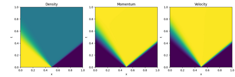
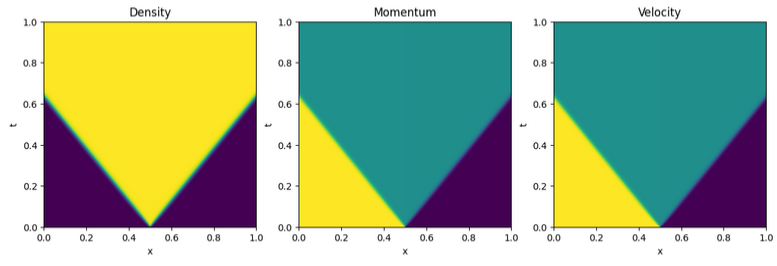
Expansion-shock. \((\rho_A, u_A) = (2, 0)\), \((\rho_B, u_B) = (1, 0)\)

Shock-shock. \((\rho_A, u_A) = (1, .5)\), \((\rho_B, u_B) = (1, -.5)\)

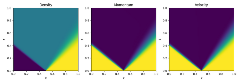
Shock-expansion. \((\rho_A, u_A) = (1, 0)\), \((\rho_B, u_B) = (2, 0)\)

Introduction to the Riemann problem

Depending on the value of the intermediate state \(\mathbf{u}_1\),

• the left wave is

  • a rarefaction wave if \(u_L < u_1\)

  • a shock wave if \(u_L > u_1\)

• the right wave is

  • a rarefaction wave if \(u_1 < u_R\)

  • a shock wave if \(u_1 > u_R\)

For two states connected by a shock wave, Rankine-Hugoniot relation holds

\[\left( u_B - u_A \right)_{1,2} = \mp a \left( \sqrt{\frac{\rho_B}{\rho_A}} - \sqrt{\frac{\rho_A}{\rho_B}} \right) \ .\]

For two states connected by an expansion wave, the following relation holds

\[(u_B- u_A)_{1,2} = \mp a \ln \frac{\rho_B}{\rho_A} \ .\]

Entropy condition

The eigenvalues of the P-sys are \(s_{1,2} = u \mp a\). Entropy condition can be summarized as:

• characteristic lines enters a shocks

• diverging characteristic lines of are connected by an exapansion fan, with a smooth solution

Solution of the Riemann problem

For simple and low-dimensional problems like P-sys, an analytical solution is feasible

Case 1. 1: shock, 2: shock. For the entropy condition, \(u_A \ge u_1 \ge u_B\).

Details

\[\begin{split}\begin{aligned} u_1 - u_A & = - a \left( \sqrt{\frac{\rho_1}{\rho_A}} - \sqrt{\frac{\rho_A}{\rho_1}} \right) \\ u_B - u_1 & = a \left( \sqrt{\frac{\rho_B}{\rho_1}} - \sqrt{\frac{\rho_1}{\rho_B}} \right) \\ \end{aligned}\end{split}\]

\[\begin{split}\begin{aligned} u_A & = u_1 + a \left( \sqrt{\frac{\rho_1}{\rho_A}} - \sqrt{\frac{\rho_A}{\rho_1}} \right) \ge u_1 \\ u_B & = u_1 + a \left( \sqrt{\frac{\rho_B}{\rho_1}} - \sqrt{\frac{\rho_1}{\rho_B}} \right) \le u_1 \\ \end{aligned}\end{split}\]

\[\begin{split}\begin{aligned} & \sqrt{\frac{\rho_1}{\rho_A}} - \sqrt{\frac{\rho_A}{\rho_1}} \ge 0 \quad \rightarrow \quad \rho_1 \ge \rho_A \\ & \sqrt{\frac{\rho_B}{\rho_1}} - \sqrt{\frac{\rho_1}{\rho_B}} \le 0 \quad \rightarrow \quad \rho_1 \ge \rho_B \\ \end{aligned}\end{split}\]

and thus \(\rho_1 \ge \max\{ \rho_A, \rho_B \}\).

Limiting cases.

\[\begin{aligned} u_A - u_B = a \left( \sqrt{\frac{\rho_1}{\rho_A}} - \sqrt{\frac{\rho_A}{\rho_1}} - \sqrt{\frac{\rho_B}{\rho_1}} + \sqrt{\frac{\rho_1}{\rho_B}} \right) \qquad (\ge 0) \end{aligned}\]

This is an increasing functon in \(\rho_1\).

If \(\rho_A \ge \rho_B\), the limiting case is \(\rho_1 = \rho_A\), i.e.

\[u_A - u_B \ge \left( u_A - u_B \right)_{\rho_1 = \rho_A} = a \left( \sqrt{\frac{\rho_A}{\rho_B}} - \sqrt{\frac{\rho_B}{\rho_A}} \right)\]

If \(\rho_B \ge \rho_A\), the limiting case is \(\rho_1 = \rho_B\), i.e.

\[u_A - u_B \ge \left( u_A - u_B \right)_{\rho_1 = \rho_B} = a \left( \sqrt{\frac{\rho_B}{\rho_A}} - \sqrt{\frac{\rho_A}{\rho_B}} \right)\]

Intermediate state. RH equations are solved for \((\rho_1, u_1)\).

…

Case 2. 1: rarefaction, 2: shock. For the entropy condition, \(u_A \le u_1\), and \(u_1 \ge u_B\).

Details

\[\begin{split}\begin{aligned} u_1 - u_A & = - a \ln \frac{\rho_1}{\rho_A} \\ u_B - u_1 & = a \left( \sqrt{\frac{\rho_B}{\rho_1}} - \sqrt{\frac{\rho_1}{\rho_B}} \right) \\ \end{aligned}\end{split}\]

\[\begin{split}\begin{aligned} u_A & = u_1 + a \ln \frac{\rho_1}{\rho_A} && \le u_1 \\ u_B & = u_1 + a \left( \sqrt{\frac{\rho_B}{\rho_1}} - \sqrt{\frac{\rho_1}{\rho_B}} \right) && \le u_1 \\ \end{aligned}\end{split}\]

\[\begin{split}\begin{aligned} \frac{\rho_1}{\rho_A} \le 1 \quad & \rightarrow \quad \rho_1 \le \rho_A \\ \sqrt{\frac{\rho_B}{\rho_1}} - \sqrt{\frac{\rho_1}{\rho_B}} \le 0 \quad & \rightarrow \quad \rho_1 \ge \rho_B \\ \end{aligned}\end{split}\]

and thus \(\rho_1 \in [\rho_B, \rho_A]\).

Limiting cases.

\[\begin{aligned} u_A - u_B = a \left( \ln \frac{\rho_1}{\rho_A} - \sqrt{\frac{\rho_B}{\rho_1}} + \sqrt{\frac{\rho_1}{\rho_B}} \right) \end{aligned}\]

This an increasing function in \(\rho_1\).

At the lower bound, \(\rho_1 = \rho_B\)

\[\begin{aligned} u_A - u_B \ge \left( u_A - u_B \right)_{\rho_1 = \rho_B } = a \ln \frac{\rho_B}{\rho_A} \end{aligned}\]

At the upper bound, \(\rho_1 = \rho_A\)

\[u_A - u_B \le \left( u_A - u_B \right)_{\rho_1 = \rho_A} = a \left( \sqrt{\frac{\rho_A}{\rho_B}} - \sqrt{\frac{\rho_B}{\rho_A}} \right)\]

Intermediate state. RH equations are solved for \((\rho_1, u_1)\).

…

Case 3. 1: shock, 2: rarefaction. Symmetric w.r.t. case 2. For the entropy condition \(u_A \ge u_1\), and \(u_1 \le u_B\).

Case 4. 1: rarefaction, 2: rarefaction. For the entropy condition \(u_A \le u_1 \le u_B\).

Details

\[\begin{split}\begin{aligned} u_1 - u_A & = - a \ln \frac{\rho_1}{\rho_A} \\ u_B - u_1 & = a \ln \frac{\rho_B}{\rho_1} \end{aligned}\end{split}\]

\[\begin{split}\begin{aligned} u_A & = u_1 + a \ln \frac{\rho_1}{\rho_A} && \le u_1 \\ u_B & = u_1 + a \ln \frac{\rho_B}{\rho_1} && \ge u_1 \\ \end{aligned}\end{split}\]

\[\begin{split}\begin{aligned} \frac{\rho_1}{\rho_A} \le 1 \quad & \rightarrow \quad \rho_1 \le \rho_A \\ \frac{\rho_B}{\rho_1} \ge 1 \quad & \rightarrow \quad \rho_1 \le \rho_B \\ \end{aligned}\end{split}\]

and thus \(\rho_1 \le \min\{\rho_A, \rho_B\}\).

Limiting cases.

\[\begin{aligned} u_A - u_B = a \left( \ln \frac{\rho_1}{\rho_A} - \ln \frac{\rho_B}{\rho_1} \right) \end{aligned}\]

This an increasing function in \(\rho_1\).

If \(\rho_A \le \rho_B\), the limiting case is \(\rho_1 = \rho_A\), i.e.

\[\begin{aligned} u_A - u_B \le \left( u_A - u_B \right)_{\rho_1 = \rho_A } = - a \ln \frac{\rho_B}{\rho_A} = a \ln \frac{\rho_A}{\rho_B} \end{aligned}\]

If \(\rho_B \le \rho_A\), the limiting case is \(\rho_1 = \rho_B\), i.e.

\[ u_A - u_B \le \left( u_A - u_B \right)_{\rho_1 = \rho_B } = a \ln \frac{\rho_B}{\rho_A} \]

Intermediate state. RH equations are solved for \((\rho_1, u_1)\).

Summary of the P-sys

Differential equations. In conservative form

\[\begin{split} \partial_t \begin{bmatrix} \rho \\ m \end{bmatrix} + \partial_x \begin{bmatrix} m \\ \frac{m^2}{\rho} + a^2 \rho \end{bmatrix} = \mathbf{0} \ , \end{split}\]

with constant speed of sound \(a\). Convective form reads

\[\begin{split} \partial_t \begin{bmatrix} \rho \\ m \end{bmatrix} + \begin{bmatrix} 0 & 1 \\ a^2 - \frac{m^2}{\rho^2} & 2 \frac{m}{\rho} \end{bmatrix} \partial_x \begin{bmatrix} \rho \\ m \end{bmatrix} = \mathbf{0} \end{split}\]

Spectral decomposition - Characteristics

Eigenvalues.

\[\begin{split}0 = |\mathbf{A} - s \mathbf{I}| = \left| \begin{bmatrix} -s & 1 \\ a^2 - u^2 & -s +2u \end{bmatrix} \right| = s ( s - 2 u ) + u^2 - a^2\end{split}\]

\[s_{1,2} = u \mp a\]

Right eigenvectors.

\[\begin{split}\mathbf{R} = \begin{bmatrix} \rho & \rho \\ \rho ( u - a ) & \rho ( u + a ) \end{bmatrix}\end{split}\]

Left eigenvectors.

\[\begin{split}\mathbf{L} = \frac{1}{2 \rho^2 a} \begin{bmatrix} \rho ( u + a ) & - \rho \\ - \rho (u-a) & \rho \end{bmatrix}\end{split}\]

Spectral decomposition.

\[\mathbf{A} = \mathbf{R} \boldsymbol{\Lambda} \mathbf{L} \ .\]

Characteristic lines and Riemann invariants. Let \(\mathbf{v}\) the characteristic variables defined by the condition \(d \mathbf{v} = \mathbf{L} d \mathbf{u}\), the PDE

\[\begin{split}\begin{aligned} \mathbf{0} & = \partial_t \mathbf{u} + \mathbf{A}(\mathbf{u}) \partial_x \mathbf{u} = \\ & = \partial_t \mathbf{u} + \mathbf{R} \boldsymbol{\Lambda} \mathbf{L} \partial_x \mathbf{u} \ , \end{aligned}\end{split}\]

after multiplying by \(\mathbf{L}\) on the left, becomes the diagonal system of equation

\[\partial_t \mathbf{v} + \boldsymbol{\Lambda} \partial_x \mathbf{v} = \mathbf{0} \ .\]

Let \(\mathbf{V}(t) = \mathbf{v}(X(t),t)\) the value of the characteristic variables on the line \(X(t)\). Exploiting the derivation of composite functions,

\[d_t \mathbf{U}(t) = \partial_t \mathbf{u}(X(t),t) + \dot{X}(t) \partial_x \mathbf{u}(X(t), t) \ ,\]

and inserting in the PDE,

\[\begin{split}\begin{aligned} 0 & = \partial_t v_i + s_i \partial_x v_i = \\ & = d_t V_i + ( s_i - \dot{X} ) \partial_x v_i \ . \end{aligned}\end{split}\]

Characteristic lines are defined by the condition \(\dot{X}_i(t) = s_i(\mathbf{U}(t))\), and on these lines \(d_t V_i = 0\), i.e. the \(i^{th}\) characteristic variable is constant on the characteristic lines of the \(i^{th}\) family. For a P-sys, characteristic lines of family 1, 2 satisfy

\[\begin{split}\begin{cases} \dot{X}_{1,2}(t) = a - u(X_{1,2}(t), t) \\ 0 = \dot{V}_{1,2} = \frac{1}{2 R^2 a} \left[ R (a \pm U) \dot{R} \mp R \dot{M} \right] = \frac{1}{2} \left[ \frac{\dot{R}}{R} \mp \frac{\dot{U}}{a} \right] = \frac{1}{2} \frac{d}{dt} \left[ \ln \left( \frac{R}{\rho_0} \right) \mp \frac{U}{a} \right] \end{cases}\end{split}\]

with \(\dot{m} = \dot{\rho} u + \rho \dot{u}\)

Integral equations. On a control volume \(V\) at rest

\[\begin{split}\begin{aligned} & \dfrac{d}{dt} \int_{V} \rho + \oint_{\partial V} \mathbf{m} \cdot \hat{\mathbf{n}} = 0 \\ & \dfrac{d}{dt} \int_{V} \mathbf{m} + \oint_{\partial V} \left[ \frac{\mathbf{m} \mathbf{m}}{\rho} + a^2 \rho \mathbb{I} \right] \cdot \hat{\mathbf{n}} = \mathbf{0} \\ \end{aligned}\end{split}\]

and for an arbitrary volume \(v_t\)

\[\begin{split}\begin{aligned} & \dfrac{d}{dt} \int_{v_t} \rho + \oint_{\partial v_t} \rho ( \mathbf{u} - \mathbf{u}_b ) \cdot \hat{\mathbf{n}} = 0 \\ & \dfrac{d}{dt} \int_{v_t} \rho \mathbf{u} + \oint_{\partial v_t} \rho \mathbf{u} \left( \mathbf{u} - \mathbf{u}_b \right) \cdot \hat{\mathbf{n}} + \oint_{\partial v_t} \rho a^2 \hat{\mathbf{n}} = \mathbf{0} \end{aligned}\end{split}\]

Jump conditions.

\[\begin{split}\begin{cases} 0 = \left[ \rho u^{rel} \right] \\ 0 = \left[ \rho u u^{rel} + \rho a^2 \right] \end{cases}\end{split}\]

Shocks

The speed of the shock can be written as a function of the physical quantities on its sides, with \(n\) different expressions, one per component of the relation

\[\dot{s} \left[ \mathbf{u} \right] = \left[ \mathbf{F}(\mathbf{u}) \right] \ ,\]

here for the P-sys

\[\begin{split}\begin{cases} \rho_1 ( u_1 - \dot{s} ) = \rho_2 ( u_2 - \dot{s} ) \\ \rho_1 ( u_1 - \dot{s} ) u_1 + \rho_1 a^2 = \rho_2 ( u_2 - \dot{s} ) u_2 + \rho_2 a^2 \end{cases}\end{split}\]

and thus

\[\begin{split}\begin{aligned} \dot{s} & = \frac{\rho_2 u_2 - \rho_1 u_1}{\rho_2 - \rho_1} = \\ & = \frac{\rho_2 ( u_2^2 + a^2 ) - \rho_1 ( u_1^2 + a^2 )}{\rho_2 u_2 - \rho_1 u_1} \ . \end{aligned}\end{split}\]

Comparing the two expressions of the speed of the shock, a relation between physical quantities on the sides of the shock appears

\[\begin{split}\begin{aligned} 0 & = ( \rho_2 u_2 - \rho_1 u_1 )^2 - ( \rho_2 - \rho_1 )( \rho_2 (u_2^2 + a^2 ) - \rho_1 (u_1^2 + a^2 ) ) = \\ & = \rho_2^2 u_2^2 - 2 \rho_1 \rho_2 u_1 u_2 + \rho_1^2 u_1^2 - \rho_2^2 (u_2^2 + a^2) - \rho_1^2 (u_1^2 + a^2) + \rho_1 \rho_2 ( u_2^2 + 2 a^2 + u_1^2 ) = \\ & = - 2 \rho_1 \rho_2 u_1 u_2 - \rho_2^2 a^2 - \rho_1^2 a^2 + \rho_1 \rho_2 ( u_2^2 + 2 a^2 + u_1^2 ) = \\ & = \rho_1 \rho_2 ( u_1 - u_2 )^2 - a^2 ( \rho_2 - \rho_1 )^2 \ , \end{aligned}\end{split}\]

and thus the Rankine-Hugoniot relation follows

\[\left( u_2 - u_1 \right)_{1,2} = \mp \frac{a}{\sqrt{\rho_1\rho_2}} ( \rho_2 - \rho_1 ) \ .\]

The speed of the shock is

\[\begin{split}\begin{aligned} \dot{s}_{1,2} & = \frac{1}{\rho_2 - \rho_1} \left[ \rho_2 \left( u_1 \mp \frac{a}{\sqrt{\rho_1 \rho_2}} (\rho_2 - \rho_1) \right) - \rho_1 u_1 \right] = \\ & = \frac{1}{\rho_2 - \rho_1} \left[ \left( \rho_2 - \rho_1 \right) u_1 \mp \rho_2 \frac{a}{\sqrt{\rho_1 \rho_2}} (\rho_2 - \rho_1) \right] = \\ & = u_1 \mp a \sqrt{\frac{\rho_2}{\rho_1}} \end{aligned}\end{split}\]

\[\begin{split}\begin{aligned} \dot{s}_{1,2} & = \frac{1}{\rho_2 - \rho_1} \left[ \rho_2 u_2 - \rho_1 \left( u_2 \pm \frac{a}{\sqrt{\rho_1 \rho_2}} (\rho_2 - \rho_1) \right) \right] = \\ & = u_2 \mp a \sqrt{\frac{\rho_1}{\rho_2}} \end{aligned}\end{split}\]

Self-similar solutions at a discontinuity in the initial state.

Self-similar solution - expansion fan

With the similarity variable

\[\xi = \frac{x}{t} \ ,\]

and the function \(\mathbf{U}(\xi) = \mathbf{u}(x, t)\),

\[\begin{split}\begin{aligned} \partial_t \mathbf{u} & = \partial_t \xi \mathbf{U}' = - \frac{x}{t^2} \mathbf{U}'(\xi) \\ \partial_x \mathbf{u} & = \partial_x \xi \mathbf{U}' = \frac{1}{t } \mathbf{U}'(\xi) \\ \end{aligned}\end{split}\]

so that the equation becomes

\[\mathbf{0} = - \xi \mathbf{U}' + \mathbf{A} \mathbf{U}' = \left[ - \xi \mathbf{I} + \mathbf{A} \right] \mathbf{U}'(\xi) \ .\]

This is an eigenvalue problem, as the trivial solution \(\mathbf{U}'(\xi) = \mathbf{0}\) can’t produce a smooth function between two discontinuous states. The solution of the eigenvalue problem reads

\[\xi_{1,2} = U(\xi) \mp a \ ,\]

with right eigenvectors

\[\begin{split}\mathbf{r}_{1,2} = \begin{bmatrix} \rho(\xi) \\ \rho(\xi) ( u(\xi) \mp a ) \end{bmatrix} \ ,\end{split}\]

These conditions define two families of expansion fans, one originating from the first family of charactersitic and one originating from the second family.

The derivative of the conservative variable w.r.t. \(\xi\) must be proportional to the right eigenvectors

\[\begin{split}\mathbf{U}'_{1,2}(\xi) = \begin{bmatrix} \rho_{1,2}' \\ m_{1,2}' \end{bmatrix} = C_{1,2} \begin{bmatrix} \rho \\ m \mp \rho a \end{bmatrix} \ ,\end{split}\]

or

\[\begin{split}\begin{cases} \rho' = C \rho \\ m' = C ( m \mp \rho a ) \end{cases}\end{split}\]

Integration gives

\[\rho_{1,2}(\xi) = \rho_A e^{C (\xi-\xi_A)}\]

and

\[m' = C m \mp C \rho_A a e^{C (\xi-\xi_A)}\]

The solution reads (see below for a very short review of the solution of this kind of ODE)

\[\begin{split}\begin{aligned} m_{1,2}(\xi) & = m_A e^{C \xi} \mp C \rho_A a \xi e^{C ( \xi - \xi_A)} = \\ & = m_A e^{C (\xi-\xi_A)} \mp C ( \xi - \xi_A ) \, a \, \rho_{1,2}(\xi) \end{aligned}\end{split}\]

Let \(m(\xi) = \rho(\xi) u(\xi)\), then the velocity field is

\[u_{1,2}(\xi) = u_A \mp C ( \xi - \xi_A ) \, a \ .\]

This expression can be recast as a function of \(u\) and \(\rho\), as \(C(\xi - \xi_A) = \ln \frac{\rho_{1,2}}{\rho_A}\), as

\[u_{1,2}(\xi) = u_a \mp a \ln \frac{\rho_{1,2}}{\rho_A} \ .\]

Solution of the 1-st order linear non-homogeneous ODE

\[y'(x) = C y(x) + A e^{Cx}\]

The solution of the homogeneous

\[y_o(x) = a e^{C x} \ ,\]

is propoprtional to the forcing. The particular solution of the non-homogeneous equation has the form

\[y_p(x) = b x e^{C x} \ ,\]

so that its derivative is

\[y'_p(x) = b e^{C x} + b C x e^{C x} \ .\]

Sostitution in the ODE gives

\[b e^{C x} + b C x e^{C x} = C \left( b x e^{Cx} \right) + A e^{Cx} \]

and thus \(b = A\). The solution of the non-homogeneous equation thus reads

\[y(x) = a e^{Cx} + A x e^{Cx} \ ,\]

with the integration constant \(a\) that is determined by a condition (initial, final, or whatever).