58.4.1. 1-dimensional P-system#
58.4.1.1. Useful classes for numerical methods#
58.4.1.1.1. Basic libraries#
Show code cell source
import numpy as np
import matplotlib.pyplot as plt
58.4.1.1.2. Parent class#
\(\texttt{HyperbolicSystem1d()}\) class with common functions (or just their templates) required to implement a finite volume method solver.
Show code cell source
class HyperbolicSystem1d():
    """
    Analytical quantities of a Hyperbolic linear system in a 1-dimensional domain
    """
    def __init(self, **params):
        pass
    def flux(self,):
        """ Analytical flux, f """
        pass
    def A(self,):
        """ Advection matrix, A """
        pass
    def s(self,):
        """ Eigenvalues of matrix, s """
        pass
    def R(self,):
        """ Matrix of right eigenvectors, R """
        pass
    def L(self,):
        """ Matrix of left eigenvectors, L=inv(R) """
        pass
    def spectrum(self,):
        """ Spectrum of matrix A() """
        return self.s(), self.R(), self.L()

    def absA(self, u):
        """ A = R * S * L, |A| = R * |S| * L """
        return self.R(u) @ np.diag(np.abs(self.s(u))) @ self.L(u)

    def roe_intermediate_state(self,):
        """ Roe intermediate state for Roe linearization """
        pass
58.4.1.1.3. P-system class#
Show code cell source
class Psys1d(HyperbolicSystem1d):
    """
    Analytical quantities of a Hyperbolic linear system in a 1-dimensional domain
    Physical quantities:
    - conservative: (rho, m)
    - physical/convective (rho, u)
    Parameters:
    - a: speed of sound
    """
    def __init__(self, a, name=""):
        """  """
        self.a = a
        self.a2 = self.a**2
        self.name = name

    def flux(self, u):
        """ Numerical flux
        u: conservative variables (rho, m)
        F = ( m, m^2/rho + rho*a^2 )
        """
        return np.array([ u[1], u[1]**2/u[0]+u[0]*self.a2])

    def A(self, u):
        """ Convection matrix, A; input: conservative variables """
        vel = u[1]/u[0]
        return np.array([[ .0, 1. ], [ -vel**2+self.a2, 2*vel]])

    def s(self, u):
        """ Eigenvalues of A; input: conservative variables """
        vel = u[1]/u[0]
        return np.array([vel-self.a, vel+self.a])

    def R(self, u):
        """ Right eigenvectors of A; input: conservative variables """
        vel = u[1]/u[0]
        return np.array([[1, vel-self.a],[1, vel+self.a]]).T

    def L(self, u):
        """ Left eigenvectors of A; input: conservative variables """
        vel = u[1]/u[0]
        return np.array([[vel+self.a, -vel+self.a],[-1., 1.]]).T / (2.*self.a)

    def spectrum(self, u):
        """ Spectrum of matrix A; input: conservative variables """
        return self.s(u), self.R(u), self.L(u)

    def roe_intermediate_state(self, u_0, u_1):
        """
        rho_roe = ANY! = ... CHOOSE ONE: average = 0.5*(rho_0+rho_1)
        vel_roe = (sqrt(rho_0)*vel_0+sqrt(rho_1)*vel_1)/(sqrt(rho_0)+sqrt(rho_1))
        - convective/physical: (rho, vel) = ( rho_roe, vel_roe )
        - conservatvie       : (rho, mom) = ( rho_roe, rho_roe*vel_roe)
        F_roe(u) ~ dFdu * du ~ A(u_roe(u0,u1)) * (u_1 - u_0)
        """
        rho_roe = .5*(u_0[0]+u_1[0])
        vel_0, vel_1 = u_0[1]/u_0[0], u_1[1]/u_1[0]
        vel_roe = (vel_0*np.sqrt(u_0[0])+vel_1*np.sqrt(u_1[0])) / \
                  (np.sqrt(u_0[0])+np.sqrt(u_1[0]))

        return np.array([rho_roe, rho_roe*vel_roe])

    def absA_entropy_fix(self, u, delta=.1):
        """  """
        #> Eigenvalues s1 = u-a, s2 = u+a
        eigvals = self.s(u)
        #> Speed of sound a = .5 * ( s2 - s1 )
        a = .5 * ( np.max(eigvals) - np.min(eigvals) )
        #> Entropy fix
        entropy_evals = np.abs(eigvals)
        entropy_evals[entropy_evals < delta*a] = \
            .5 * entropy_evals[entropy_evals < delta*a]**2 / ( delta * a ) + .5 * ( delta * a )

        return  self.R(u) @ np.diag(entropy_evals) @ self.L(u)

    def roe_flux(self, u_0, u_1):
        """  """
        u_roe = self.roe_intermediate_state(u_0, u_1)

        return .5 * (self.flux(u_1) + self.flux(u_0) + \
                     self.absA(u_roe) @ ( u_0 - u_1 ) )

    def flux_at_boundary(self, boundary, u):
        """
        boundary: boundary conditino dict
        u: conservative variables (rho, m, Et) at boundary cell
        """

        if ( boundary["type"] == "wall" ):
            u_boundary = u.copy(); u_boundary[1] = -u[1]
            if ( boundary["nor"] < 0 ):
                return self.roe_flux(u_boundary, u)
            else:
                return self.roe_flux(u, u_boundary)

        elif ( boundary["type"] == "inflow" or boundary["type"] == "outflow" ):
            delta_v = self.L(u) @ ( self.cons_from_phys(boundary["phys_ext"]) - u )
            eigval = self.s(u)
            delta_v[ eigval*boundary["nor"] > 0 ] = .0
            u_flux = u + self.R(u) @ delta_v

            return self.flux(u_flux)
58.4.1.2. Numerical simulation#
58.4.1.2.1. System of equations#
Initialized the system of equations to be solved
Show code cell source
#> P-system
# Number of unknown fields, nu
# - conservative       : u = (rho, mom)
# - physical/convective: p = (rho, vel), with mom = rho*vel
nu = 2

#> Parameters and initialization of the system
a = 1.               # speed of sound
S = Psys1d(a)
# S = ShallowWater1d(g=1)
# S = Psys1dLinearized(a)
# S = Euler1dPIG(...)
58.4.1.2.2. Domain#
Show code cell source
#> Parameters
x0, x1 = 0., 1.                          # coords of left and right boundaries
ne = 200                                 # n. of elements

#> Domain
xs = np.linspace(x0, x1, ne+1)           # coord of the cell boundaries
xc = .5 * ( xs[:-1] + xs[1:] )           # coord of the cell centers
dx = xs[1:] - xs[:-1]                    # volume of the cells

#> Initial condition of a Riemann problem
# ES, SS, SE, EE
rhoL, rhoR = 1., 1.
uL, uR = -.5, .5
58.4.1.2.3. Boundary conditions#
Show code cell source
# boundary_0 = {  # left boundary
#     "type": "wall",
#     "nor" : -1.
# }
# boundary_1 = {  # right boundary
#     "type": "wall",
#     "nor" : 1.
# }
boundary_0 = {  # left boundary
    "type": "inflow",
    "phys_ext": np.array([rhoL, uL]),      # rho_ext, u_ext
    "nor": -1.                             # nx
}
boundary_1 = {  # right boundary
    "type": "outflow",
    "phys_ext": np.array([rhoR, uR]),      # rho_ext, u_ext
    "nor": 1.                              # nx
}
58.4.1.2.4. Simulation parameters#
Show code cell source
#> Time
t0, t1, dt = 0., 1., .00125
nt = int((t1-t0)/dt)+1
tv = np.arange(nt)*dt

#> Boundary conditions
u0_fun = lambda t: np.array([0., 0.])
u1_fun = lambda t: np.array([0., 0.])

#> Initial boundary conditions
uc0 = np.zeros((nu,ne))
uc0[0,:] = np.where( xc<.5, rhoL, rhoR )
uc0[1,:] = np.where( xc<.5, rhoL*uL, rhoR*uR )
# uc0[0,:] = 1.
# uc0[1,:] = np.where( xc<.5, .1, -.1)
# uc0[0,:] = 1. + .2 * xc / (x1-x0)
# uc0[1,:] = 0.
58.4.1.2.5. Time loop#
Show code cell source
#> Numerical schemes
#> Time integration
time_integration = 'ee'       # ...
numerical_flux   = 'roe'      # ...

"""
#> Boundary condiitons
u0_wall = lambda t: .0 * np.sin(2*np.pi*t)   # vel at solid wall
u1_wall = lambda t: .0 * np.sin(2*np.pi*t)   # vel at solid wall
r1_free = lambda t: .1 # .0 * np.sin(2*np.pi*t)   # rho at free wall
"""

#> Time loop
it = 0
uuc = np.zeros((nt, nu, ne))    # Array to store solution, for small dimensional pbs
uc = uc0.copy()
uuc[0,:,:] = uc

# print(uc)
u_0, u_1 = uc[:,0].copy(), uc[:,-1].copy()  # extrapolated states

while it < nt-1:

    t = tv[it]

    #> Evaluate fluxes at internal boundaries
    if numerical_flux == 'roe':
        flux = np.array([ S.roe_flux(uc[:,ia], uc[:,ia+1]) for ia in range(ne-1) ]).T

    #> Flux at boundaries
    flux_0 = S.roe_flux(u_0, uc[:,0])
    flux_1 = S.roe_flux(uc[:,-1], u_1)
    # Bcs...correction after the solution have been evaluated?

    # flux = np.append(np.append(flux_0, flux), flux_1)
    flux = np.concatenate((flux_0[:,np.newaxis], flux, flux_1[:, np.newaxis]), axis=1)


    #> Time integration
    if time_integration == 'ee':
        dt = tv[it+1] - tv[it]
        uc += ( flux[:,:-1] - flux[:,1:] ) * dt / dx

    it += 1                   # Updating counter
    uuc[it,:,:] = uc.copy()   # Storing results
58.4.1.2.6. Post-processing#
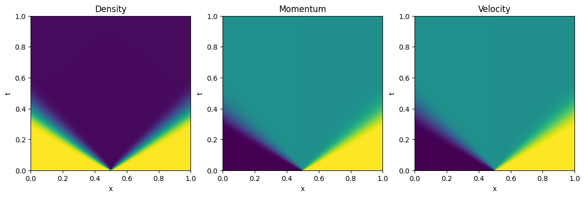
Show code cell source
fig, ax = plt.subplots(1,3, figsize=(14, 4))

iax = 0
ax[iax].imshow(uuc[:,0,:], aspect="auto", extent=[x0, x1, t1, t0])
# ax[0].set_colorbar()
ax[iax].set_xlabel('x')
ax[iax].set_ylabel('t')
ax[iax].set_title('Density')
ax[iax].invert_yaxis()

iax = 1
ax[iax].imshow(uuc[:,1,:], aspect="auto", extent=[x0, x1, t1, t0])
# ax[0].set_colorbar()
ax[iax].set_xlabel('x')
ax[iax].set_ylabel('t')
ax[iax].set_title('Momentum')
ax[iax].invert_yaxis()

iax = 2
ax[iax].imshow(uuc[:,1,:]/uuc[:,0,:], aspect="auto", extent=[x0, x1, t1, t0])
# ax[0].set_colorbar()
ax[2].set_xlabel('x')
ax[iax].set_ylabel('t')
ax[iax].set_title('Velocity')
ax[iax].invert_yaxis()
Show code cell source
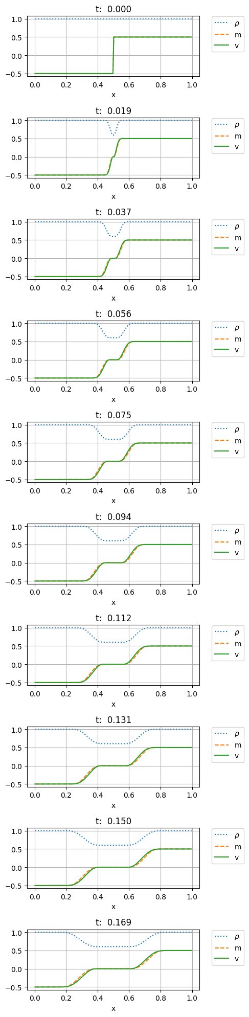
fig, ax = plt.subplots(10, figsize=(5,20))
for i in range(10):
    ax[i].plot(xc,uuc[15*i,0,:], ':' , label=r'$\rho$')
    ax[i].plot(xc,uuc[15*i,1,:], '--', label='m')
    ax[i].plot(xc,uuc[15*i,1,:]/uuc[15*i,0,:], '-', label='v')
    ax[i].set_xlabel('x')
    ax[i].set_title(f"t: {15*i*dt:6.3f}")

    ax[i].grid()
    ax[i].legend(bbox_to_anchor=(1.05, 1.05), loc='upper left')

plt.tight_layout()