29.3. Stability of integration schemes

29.3.1. Stability of a first-order linear system

Linear homogeneous equation (or system?)

\[\begin{split}\begin{aligned} \dot{y} & = \lambda y \\ y(0) & = y_0 \ , \end{aligned}\end{split}\]

is a first test for the stability of a numerical method. The problem has the exact solution

\[y(t) = y_0 e^{\lambda t} \ ,\]

and is asymptotically stable if \(\text{re}\{\lambda\} < 0\), as

\[\lim_{t \rightarrow +\infty} y(t) = \lim_{t \rightarrow +\infty} y_0 e^{\lambda t} = \lim_{t \rightarrow +\infty} y_0 e^{\text{re}\{\lambda\} t} e^{j \, \text{im}\{\lambda\} t} \ . \]

Forced linear equation (or system?)

\[\dot{y} = \lambda y + u \ .\]

The exact solution converges to the forced solution if the system is asymptotically stable, For periodic forcing, the behavior can be evaluated in frequency (Laplace or Fourier) domain

\[y(s) = \frac{1}{s - \lambda} u(s) \ .\]

29.3.1.1. A-stability

A-stability ensures the numerical method doesn’t explode in the simulation of a asymptotically stable system.

A numerical method is defined A-stable if its stability region includes the whole left half plane.

29.3.1.2. L-stability

Let \(z := h \lambda\). For one-step methods, it’s possible to define a scalar transfer function \(G(z)\) between \(y_{n}\) and \(y_{n+1}\),

\[y_{n+1} = G(z) y_n \ .\]

For multi-step methods… proerties of characteristic polynomial and its roots

For systems… amplification matrix…

L-stability ensures that the method damps extremely fast - stiff - modes, that are usually physically irrelevant but that can be numerically troublesome. A method is defined L-stable if

\[\lim_{z \rightarrow -\infty} G(z) = 0 \ .\]

29.3.1.3. 0-stability

0-stability (of a numerical method for a certain differential equation on a given interval) if a perturbation in the starting value of size \(\varepsilon\) causes the numerical solution over the time interval to change less than \(K \varepsilon\) for some \(K\) that doesn’t depend on the time-step \(h\).

It’s enough to check the conditions for the differential equation \(y' = 0\) todo why? check it!

A linear multi-step method is zero-stable iif the root condition (analogous to at least marginally stable system, i.e. roots with absolute value \(|z| < 1\), or \(|z| = 1\) with multiplicity \(= 1\)) is satisfied.

29.3.2. Some schemes

29.3.2.1. Homogeneous equation

\[\dot{y} = f(t,y) = \lambda y \ .\]

Explicit Euler.

\[y_{n+1} = y_{n} + h f(y_n, t_n) = y_n + h \lambda y_n = ( 1 + h \lambda ) y_n \ .\]

The solution of this difference equation with initial condition \(y_0\) reads

\[y_{n} = ( 1 + h \lambda )^n y_0 \ .\]

Implicit Euler.

\[y_{n+1} = y_{n} + h f(y_{n+1}, t_{n+1}) = y_n + h \lambda y_{n+1} \ .\]

The solution of this difference equation with initial condition \(y_0\) reads

\[y_{n} = \frac{1}{( 1 - h \lambda )^n} y_0 \ .\]

Crank-Nicolson.

\[y_{n+1} = y_n + \frac{h}{2} \left[ f(y_{n}, t_{n}) + f(y_{n+1}, t_{n+1}) \right] = y_n + \frac{h}{2} \left[ \lambda y_{n} + \lambda y_{n+1} \right] \ .\]

\[y_{n} = \left[ \frac{1 + \lambda h / 2}{1 - \lambda h / 2} \right]^n y_0 \ .\]

BDF 2. BDF 2 is a multi-step approach, so either \(Z\)-transform of the conversion to a one-step 2-dimensional system is required to discuss its stability properties, and transfer function.

\[y_{n+1} - \frac{4}{3} y_{n} + \frac{1}{3} y_{n-1} = \frac{2}{3} h f(t_{n+1}, y_{n+1}) \]

\[y_{n+1} - \frac{4}{3} y_{n} + \frac{1}{3} y_{n-1} = \frac{2}{3} h \lambda y_{n+1} \]

Z-transform. Using the definition \(\zeta := \lambda h\), and applying the \(Z\)-transform,

\[\begin{split}\begin{aligned} 0 & = \left[ \left( 1 - \frac{2}{3} z \right) - \frac{4}{3} \zeta^{-1} + \frac{1}{3} \zeta^{-2} \right] Y(\zeta) \\ \end{aligned}\end{split}\]

the characteristic polynomial reads

\[\begin{aligned} 0 & = \pi(\zeta; z) = \left( 3 - 2 z \right) \zeta ^2 - 4 \zeta + 1 \ . \end{aligned}\]

The roots of the polynomial depend on \(z \in \mathbb{C}\), and the system is stable if all the roots have \(|\zeta_k| \le 1\). This condition can be summarized with the condition of spectral radius of the matrix \(\mathbf{A}\) of the one-step system, \(\rho(\mathbf{A}) = \max |\lambda_k| < 1\).

Reduction of difference equation to a one-step system. The 2-step difference equation above

\[y_{n+1} - \frac{4}{3 - 2 z} y_{n} + \frac{1}{3 - 2 z} y_{n} = 0\]

can be recast as a system, \(y_n = z_{1,n}\), \(y_{n-1} = z_{0,n}\)

\[\begin{split}\begin{aligned} z_{0,n+1} & = z_{1,n} \\ z_{1,n+1} & = \frac{4}{3 - 2 z} z_{1,n} - \frac{1}{3 - 2 z} z_{0,n} \end{aligned}\end{split}\]

or using matrix formalism

\[\mathbf{z}_{n+1} = \mathbf{A} \mathbf{z}_n \ ,\]

with \(\mathbf{A} = \begin{bmatrix} \cdot & 1 \\ -\frac{1}{3 - 2 z} & \frac{4}{3 - 2 z} \end{bmatrix}\). The eigenvalues of the system follows from the condition

\[0 = \zeta \left( \zeta - \frac{4}{3 - 2 z} \right) + \frac{1}{3-2 z} \ , \]

i.e. the same condition as \(\pi(\zeta; z) = 0\).

L-stability. As \(\rightarrow +\infty\), the polynomials goes to \(\pi(z \rightarrow + \infty; \zeta) \sim - \frac{2}{3} z \zeta^2\) and thus the roots goes to \(z \rightarrow + \infty\).

Methods for second-order equations.

\[\ddot{\mathbf{x}} = \mathbf{f}(t, \mathbf{x}) \ ,\]

or as a first-order system

\[\begin{split}\begin{bmatrix} \dot{\mathbf{x}} \\ \dot{\mathbf{v}} \end{bmatrix} = \begin{bmatrix} \mathbf{v} \\ \mathbf{f}(\mathbf{x},t) \end{bmatrix} \ .\end{split}\]

A test second-order homogeneous equation may be the dynamical equation of an undapmed mass-spring system,

\[\ddot{x} + \Omega^2 x = 0 \ ,\]

being \(( d_t + i \Omega )( d_t - i \Omega ) x = 0\). This analysis can be performed with a system with conjugate complex eigenvalues \(\lambda = \sigma + j \omega\) and \(\lambda^* = \sigma - j \omega\), sot that the test equation becomes

\[\begin{split}\begin{aligned} 0 & = ( d_t - \sigma - i \omega )( d_t - \sigma + i \omega ) x = \\ & = d_{tt} x - 2 \sigma d_t x + ( \sigma^2 + \omega^2 ) \ . \end{aligned}\end{split}\]

Leapfrog method.

\[\begin{split}\left\{\begin{aligned} x_{i+1} & = x_i + h v_i + \frac{h^2}{2} f(x_i) \\ v_{i+1} & = v_i + \frac{h}{2} \left( f(x_i) + f(x_{i+1}) \right) \ . \end{aligned}\right.\end{split}\]

Verlet method. Position Verlet is algebrically equivalent to the Leapfrom method, so it shares the same stability properties.

Newmark method. …

Test equation has \(f(x) = - \Omega^2 x\), so that Leapfrog method applied to the test problem reads

\[\begin{split}\left\{\begin{aligned} x_{i+1} & = x_i + h v_i - \frac{h^2 \Omega^2}{2} x_i\\ v_{i+1} & = v_i - \Omega^2 \frac{h}{2} \left(x_i + x_{i+1} \right) \ . \end{aligned}\right.\end{split}\]

so that the \(\mathbf{z}_{i+1}\) state can be written as a function of the \(\mathbf{z}_i\) state

\[\begin{split}\begin{bmatrix} 1 & \cdot \\ \frac{h \Omega^2}{2} & 1 \end{bmatrix} \begin{bmatrix} x \\ v \end{bmatrix}_{i+1} = \begin{bmatrix} 1 - \frac{h^2 \Omega^2}{2} & h \\ -\frac{h \Omega^2}{2} & 1 \end{bmatrix} \begin{bmatrix} x \\ v \end{bmatrix}_i\end{split}\]

or

\[\begin{split}\begin{aligned} \begin{bmatrix} x \\ h v \end{bmatrix}_{i+1} & = \begin{bmatrix} 1 & \cdot \\ -\frac{h \Omega^2}{2} & 1 \end{bmatrix} \begin{bmatrix} 1 - \frac{h^2 \Omega^2}{2} & 1 \\ -\frac{h^2 \Omega^2}{2} & 1 \end{bmatrix} \begin{bmatrix} x \\ h v \end{bmatrix}_i = \\ & = \begin{bmatrix} 1 - \frac{h^2 \Omega^2}{2} & 1 \\ - h^2 \Omega^2 \left( 1 - \frac{h^2 \Omega^2}{4} \right) & 1-\frac{h^2 \Omega^2}{2} \end{bmatrix} \begin{bmatrix} x \\ h v \end{bmatrix}_i \ . \end{aligned}\end{split}\]

Generalized test equation - with general pair of complex eigenvalues, not only imaginary eigenvalues - has \(f(x,v) = 2 \sigma v - ( \sigma^2 + \omega^2) x = - 2 \xi \Omega v - \Omega^2 x\), with

\[\begin{split}\begin{aligned} \Omega^2 & = \sigma^2 + \omega^2 \\ \sigma & = - \xi \Omega \qquad \rightarrow \qquad \xi = -\frac{\sigma}{\Omega} = - \frac{\sigma}{\sqrt{\sigma^2 + \omega^2}} \\ \end{aligned}\end{split}\]

Leapfrog method applied to the test problem reads

\[\begin{split}\left\{\begin{aligned} x_{i+1} & = x_i + h v_i + \frac{h^2 }{2} \left( - \Omega^2 x_i - 2 \xi \Omega v_i \right)\\ v_{i+1} & = v_i + \frac{h}{2} \left[ -\Omega^2 \left(x_i + x_{i+1} \right) - 2 \xi \Omega \left(v_i + v_{i+1} \right) \right] \ . \end{aligned}\right.\end{split}\]

todo check!

\[\begin{split}\begin{bmatrix} 1 & \cdot \\ \frac{h^2 \Omega^2}{2} & 1 + \xi h \Omega \end{bmatrix} \begin{bmatrix} x \\ h v \end{bmatrix}_{i+1} = \begin{bmatrix} 1 - \frac{h^2 \Omega^2}{2} & 1 - \xi h \Omega \\ -\frac{h^2 \Omega^2}{2} & 1 - \xi h \Omega \end{bmatrix} \begin{bmatrix} x \\ h v \end{bmatrix}_i\end{split}\]

\[\begin{split}\begin{aligned} \begin{bmatrix} x \\ h v \end{bmatrix}_{i+1} & = \begin{bmatrix} 1 & \cdot \\ -\frac{h^2 \Omega^2}{2 (1+\xi h \Omega)} & \frac{1}{1+\xi h \Omega} \end{bmatrix} \begin{bmatrix} 1 - \frac{h^2 \Omega^2}{2} & 1 - \xi h \Omega \\ -\frac{h^2 \Omega^2}{2} & 1 - \xi h \Omega \end{bmatrix} \begin{bmatrix} x \\ h v \end{bmatrix}_i = \\ & = \begin{bmatrix} 1 - \frac{h^2 \Omega^2}{2} & 1 - \xi h \Omega \\ - \frac{h^2 \Omega^2}{1+\xi h \Omega} \left( 1 - \frac{h^2 \Omega^2}{4} \right) & \frac{1 - \xi h \Omega}{1 + \xi h \Omega} \left( 1-\frac{h^2 \Omega^2}{2} \right) \end{bmatrix} \begin{bmatrix} x \\ h v \end{bmatrix}_i \ . \end{aligned}\end{split}\]

• if \(\xi^2 \ge 1\), then the eigenvalues are real

• if \(\xi^2 \le 1\), then the eigenvalues are conjugate complex, \(s_{1,2} = -\xi \Omega \mp j \Omega \sqrt{1 - \xi^2}\)

29.3.2.2. Forced equation

…

29.3.2.3. A-stability

Show code cell source Hide code cell source

import numpy as np
import matplotlib.pyplot as plt

ampl_fun_ee = lambda z: 1 + z
ampl_fun_ie = lambda z: 1 / ( 1 - z )
ampl_fun_cn = lambda z: ( 1 + z/2 ) / ( 1 - z/2 )

A_bdf2 = lambda z: np.array([[.0, 1.], [-1/(3-2*z), 4/(3-2*z)]])

def ampl_A_fun(z, A_fun):
    evals = np.linalg.eigvals(A_fun(z))
    ieval = np.argmax(np.absolute(evals)) # , keepdims=True)
    
    return evals[ieval]  # [0]]

def A_lf(z):
    sigh, omh = np.real(z), np.imag(z)

    bh = - sigh
    ch2 = sigh**2 + omh**2

    n1 = 1. - bh
    n2 = 1. - ch2/2.
    n4 = 1. - ch2/4.
    d1 = 1 + bh
    
    return np.array([[n2, n1], [-ch2*n4/d1, n1/d1*n2]])
    

ampl_fun_bdf2 = lambda z: ampl_A_fun(z, A_bdf2)
ampl_fun_lf   = lambda z: ampl_A_fun(z, A_lf)

ampl_fun_lf_2 = lambda z: np.max(np.absolute(np.linalg.eigvals(A_lf(z))))

ampl_funs = {
    'EE': ampl_fun_ee,
    'IE': ampl_fun_ie,
    'CN': ampl_fun_cn,
    'BDF2': ampl_fun_bdf2,
    'Leapfrog': ampl_fun_lf,
}
n_methods = len(ampl_funs)

def complex_amplification_fun(ampl_fun):
    x = np.linspace(-5.001, 5.001, 200)
    y = np.linspace(-5.001, 5.001, 200)
    X, Y = np.meshgrid(x, y)
    Z = X + 1j*Y

    return X,Y, np.vectorize(ampl_fun, otypes=[complex])(Z)

Show code cell source Hide code cell source

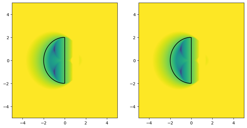
#> Check lf functions
# part of the debug. np.vectorize require otypes, otherwise some bad silent casting may occur

X, Y, Z1 = complex_amplification_fun(ampl_fun_lf)
X, Y, Z2 = complex_amplification_fun(ampl_fun_lf_2)

print(np.shape(Z1))
print(np.shape(Z2))

fig, ax = plt.subplots(1,2, figsize=(10,5))
ax[0].contour(X, Y, np.absolute(Z1), levels=[1.0], colors='black')
ax[1].contour(X, Y, np.absolute(Z2), levels=[1.0], colors='black')

ax[0].pcolormesh(X, Y, np.log(np.abs(Z1)), shading='gouraud', vmin=-3, vmax=1.)
ax[1].pcolormesh(X, Y, np.log(np.abs(Z2)), shading='gouraud', vmin=-3, vmax=1.)

plt.show()

Show code cell output Hide code cell output

(200, 200)
(200, 200)

Show code cell source Hide code cell source

#> Functions for integration of the test equation, for stability analysis of different integration schemes
def integrate_test_ee(lam, x0, tv,):
    dt = tv[1] - tv[0]
    nt = len(tv)
    xx = np.zeros(nt, dtype=complex);   xx[0] = x0

    for it in np.arange(len(tv)-1):
        xx[it+1] = ( 1. + dt * lam ) * xx[it]

    return xx


def integrate_test_ie(lam, x0, tv,):
    dt = tv[1] - tv[0]
    nt = len(tv)
    xx = np.zeros(nt, dtype=complex);  xx[0] = x0

    for it in np.arange(len(tv)-1):
        xx[it+1] = xx[it] / ( 1. - dt * lam )

    return xx


def integrate_test_cn(lam, x0, tv,):
    dt = tv[1] - tv[0]
    nt = len(tv)
    xx = np.zeros(nt, dtype=complex);   xx[0] = x0

    for it in np.arange(len(tv)-1):
        xx[it+1] = xx[it] * ( 1. + dt * lam/2 ) / ( 1. - dt * lam/2 )

    return xx


def integrate_test_bdf2(lam, x0, tv,):
    dt = tv[1] - tv[0]
    nt = len(tv)
    xx = np.zeros(nt, dtype=complex);   xx[0] = x0

    #> First step: implicit Euler
    xx[1] = xx[0] / ( 1 - dt * lam )
     
    for it in np.arange(len(tv)-1):
        xx[it+1] = ( 4*xx[it] - xx[it-1] ) / ( 3 - 2 * dt * lam )

    return xx


def integrate_test_leapfrog(lam, z0, tv,):

    sig, om = np.real(lam), np.imag(lam)
    b = - sig
    c = sig**2 + om**2
    
    dt = tv[1] - tv[0]
    nt = len(tv)
    
    xx = np.zeros(nt, dtype=complex);   xx[0] = z0[0]
    vv = np.zeros(nt, dtype=complex);   vv[0] = z0[1]

    for it in np.arange(len(tv)-1):
        xx[it+1] = xx[it] + dt * vv[it] + dt**2 / 2 * ( -2*b * vv[it] - c * xx[it] )
        vv[it+1] = ( vv[it] + dt/2 * ( -c* ( xx[it] + xx[it+1] ) - 2*b * vv[it] ) ) / ( 1 + b * dt )
    
    return xx

Show code cell source Hide code cell source

#> Perform integration in time, for different methods, for different values of z=lam*dt in the test equations
from tqdm import tqdm

dt, nt = 1., 100
tv = np.arange(nt) * dt

nz_real = 17
nz_imag = 17
z_real = np.linspace(-5.123, 5.123, nz_real)
z_imag = np.linspace(-5.123, 5.123, nz_imag)

Zreal, Zimag = np.meshgrid(z_real, z_imag)

XX = { k: {  } for k in ampl_funs.keys() }

XX['EE'  ] = { 'ic': 1., 'fun': integrate_test_ee, }
XX['IE'  ] = { 'ic': 1., 'fun': integrate_test_ie, }
XX['CN'  ] = { 'ic': 1., 'fun': integrate_test_cn, }
XX['BDF2'] = { 'ic': 1., 'fun': integrate_test_bdf2, }
XX['Leapfrog'] = { 'ic': [ 1., .0 ], 'fun': integrate_test_leapfrog, }
# XX['Leapfrog_2'] = { 'ic': [ 1., .0 ], 'fun': integrate_test_leapfrog, }

for k in XX:
     XX[k]['stability'] = np.zeros((nz_real, nz_imag))

#> Numerical integration of test equation
for method in XX:
    integrate_test = XX[method]['fun']
    x0 = XX[method]['ic']

    i_imag = 0
    for zi in z_imag:
        i_real = 0
        for zr in z_real:
            z = zr + 1j * zi
    
            xx = integrate_test(z, x0, tv)
            
            #> Check if diverging or not
            if ( np.max(np.abs(xx)) > 1.001 ):
                XX[method]['stability'][i_imag, i_real] = 0
            else:
                XX[method]['stability'][i_imag, i_real] = 1
 
            i_real += 1
        
        i_imag += 1

Show code cell source Hide code cell source

#> Plot analytical boundary of stability regions, with scatter of stability from direct integration in time
ncols = 3
nrows = ( n_methods - 1 ) // ncols + 1

fig, ax = plt.subplots(nrows, ncols, figsize=(ncols*3, nrows*3))

i_method = 0
for label, fun in ampl_funs.items():

    irow = i_method // ncols
    icol = i_method % ncols

    X, Y, G = complex_amplification_fun(fun)
    
    ax[irow, icol].contour(X, Y, np.absolute(G), levels=[1.0], colors='r')
    ax[irow, icol].contourf(X, Y, np.absolute(G), levels=[0., 1.0], colors=['#ffcccc'])
    ax[irow, icol].set_title(f"Method: {label}")
    ax[irow, icol].set_aspect("equal")
    ax[irow, icol].set_xlabel(f"Re(z)"); ax[irow, icol].set_ylabel(f"Im(z)"); ax[irow, icol].grid()

    #>
    stable_mask = ( XX[label]['stability'] == 1 )
    unstable_mask = ( XX[label]['stability'] == 0 )
    
    ax[irow, icol].scatter( Zreal[stable_mask], 
                            Zimag[stable_mask],
                            s=2, color='red', label='Stable')
   
    ax[irow, icol].scatter( Zreal[unstable_mask], 
                            Zimag[unstable_mask],
                            s=2, color='blue', label='Unstable')
    
    i_method += 1  


fig.suptitle("Stability regions of numerical methods. |G(z)| < 1")
fig.tight_layout()
# plt.axhline(0, color='black', lw=1)
# plt.axvline(0, color='black', lw=1)
# plt.grid(True, linestyle='--')
plt.show()

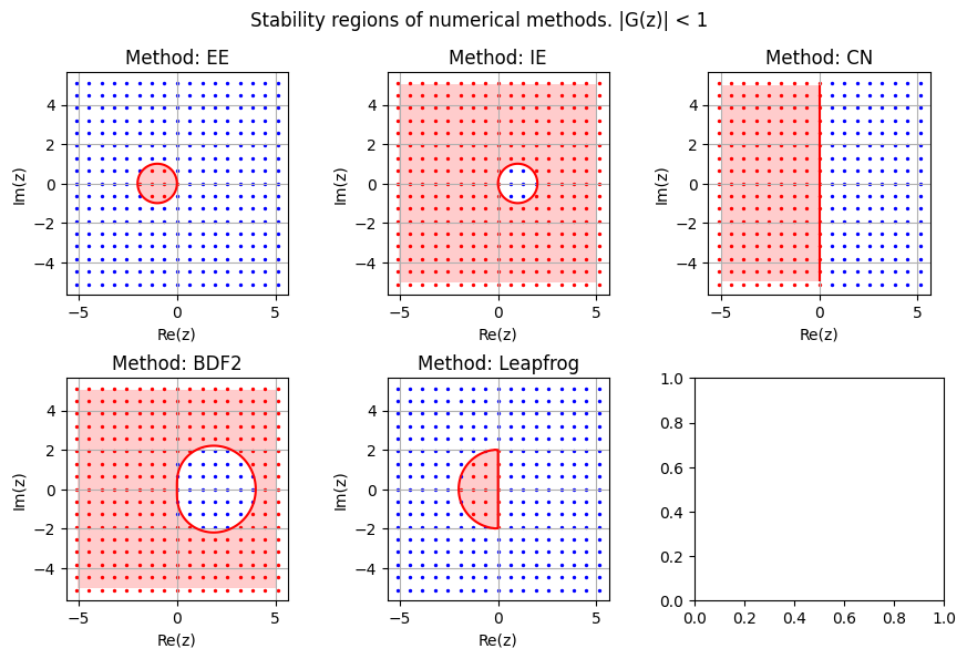
A-stability. Implicit Euler and Crank-Nicolson methods are A-stable, while explicit Euler is not.

29.3.2.3.1. G(z): absolute value and phase

Show code cell source Hide code cell source

"""
ampl_fun_bdf2 = lambda z: np.max(np.abs(np.linalg.eigvals(A_bdf2(z))))    
ampl_fun_lf = lambda z: np.max(np.abs(np.linalg.eigvals(A_lf(z))))

ampl_funs = {
    'EE': ampl_fun_ee,
    'IE': ampl_fun_ie,
    'CN': ampl_fun_cn,
    'BDF2': ampl_fun_bdf2,
    'Leapfrog': ampl_fun_lf
}
n_methods = len(ampl_funs)

"""

#> 
ncols = 3
nrows = ( n_methods - 1 ) // ncols + 1

fig, ax = plt.subplots(nrows, ncols, figsize=(ncols*3, nrows*3))

i_method = 0
for label, fun in ampl_funs.items():

    irow = i_method // ncols
    icol = i_method % ncols

    X, Y, G = complex_amplification_fun(fun)
    ax[irow, icol].contour(X, Y, np.absolute(G), levels=[1.0], colors='black')
    # ax[irow, icol].contourf(X, Y, np.abs(G), levels=[0., 1.0], colors=['#ffcccc'])
    ax[irow, icol].pcolormesh(X, Y, np.log(np.absolute(G)), cmap='hsv', shading='gouraud', vmin=-3, vmax=1.)
    ax[irow, icol].set_title(f"Method: {label}")
    ax[irow, icol].set_aspect("equal")
    ax[irow, icol].set_xlabel(f"Re(z)"); ax[irow, icol].set_ylabel(f"Im(z)"); ax[irow, icol].grid()

    i_method += 1

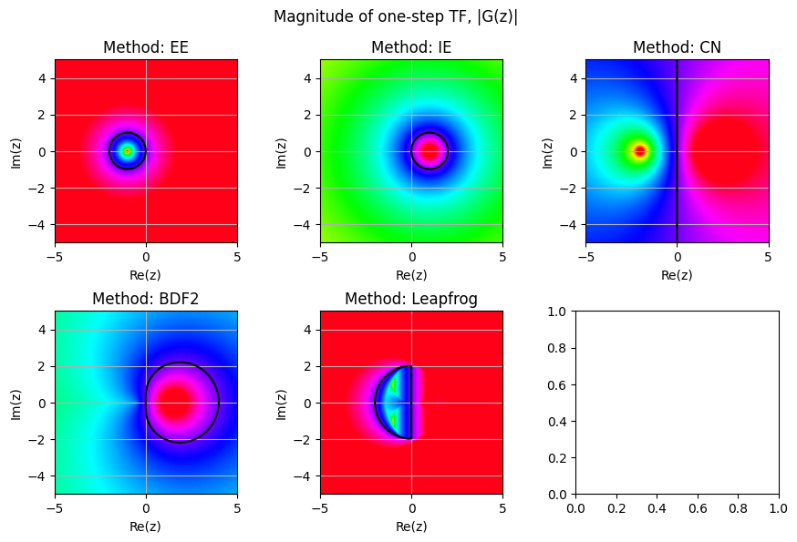
fig.suptitle("Magnitude of one-step TF, |G(z)|")
fig.tight_layout()
# plt.axhline(0, color='black', lw=1)
# plt.axvline(0, color='black', lw=1)
# plt.grid(True, linestyle='--')
plt.show()

Show code cell source Hide code cell source

fig, ax = plt.subplots(nrows, ncols, figsize=(ncols*3, nrows*3))

i_method = 0
for label, fun in ampl_funs.items():

    irow = i_method // ncols
    icol = i_method % ncols

    X, Y, G = complex_amplification_fun(fun)
    ax[irow, icol].contour(X, Y, np.abs(G), levels=[1.0], colors='black')
    # ax[irow, icol].contourf(X, Y, np.abs(G), levels=[0., 1.0], colors=['#ffcccc'])
    ax[irow, icol].pcolormesh(X, Y, np.angle(G), cmap='hsv', shading='gouraud', vmin=-np.pi, vmax=np.pi)
    ax[irow, icol].set_title(f"Method: {label}")
    ax[irow, icol].set_aspect("equal")
    ax[irow, icol].set_xlabel(f"Re(z)"); ax[irow, icol].set_ylabel(f"Im(z)"); ax[irow, icol].grid()

    i_method += 1

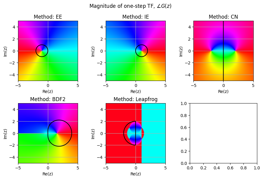
fig.suptitle(r"Magnitude of one-step TF, $\angle G(z)$")
fig.tight_layout()
# plt.axhline(0, color='black', lw=1)
# plt.axvline(0, color='black', lw=1)
# plt.grid(True, linestyle='--')
plt.show()

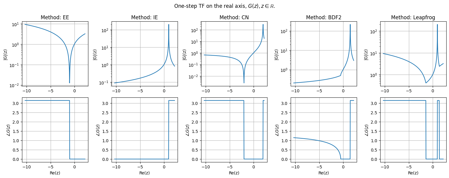
29.3.2.3.2. G(z) on the real axis

Show code cell source Hide code cell source

fig, ax = plt.subplots(2,n_methods, figsize=(n_methods*3, 2*3))
i_method = 0

for label, fun in ampl_funs.items():

    x = np.linspace(-10.34324, 2.2343242, 400)
    G = np.vectorize(fun)(x)
    
    ax[0,i_method].plot(x, np.abs(G))
    ax[0,i_method].set_title(f"Method: {label}")
    ax[0,i_method].set_ylabel(f"|G|(z)"); ax[0,i_method].grid()
    ax[0,i_method].set_yscale("log")
    ax[1,i_method].plot(x, np.angle(G))
    ax[1,i_method].set_ylabel(r"$\angle G(z)$"); ax[1,i_method].grid()
    ax[1,i_method].set_xlabel(f"Re(z)"); 

    i_method += 1

fig.suptitle(r"One-step TF on the real axis, $G(z), z \in \mathbb{R}$.")
fig.tight_layout()
plt.show()

29.3.2.3.3. G(z) on the imaginary axis

Show code cell source Hide code cell source

fig, ax = plt.subplots(2,n_methods, figsize=(n_methods*3, 2*3))
i_method = 0


min_absGs, max_absGs = [], []

for label, fun in ampl_funs.items():

    y = np.logspace(-4.3423, 4.32432, 400)
    G = np.vectorize(fun)(1j * y)

    min_absGs += [ np.min(np.abs(G)) ]
    max_absGs += [ np.max(np.abs(G)) ]
    
    ax[0,i_method].plot(y, np.abs(G))
    ax[0,i_method].set_title(f"Method: {label}")
    ax[0,i_method].set_ylabel(f"|G|(z)"); ax[0,i_method].grid()
    ax[0,i_method].set_yscale("log")
    ax[1,i_method].plot(y, np.angle(G) * 180/np.pi)
    ax[1,i_method].set_ylabel(r"$\angle G(z)$"); ax[1,i_method].grid()
    ax[1,i_method].set_xlabel(f"Re(z)");

    ax[0,i_method].set_xscale("log");  ax[1,i_method].set_xscale("log")

    i_method += 1

min_absG = np.min(min_absGs)
max_absG = np.max(max_absGs)

for i in np.arange(i_method):
    ax[0,i].set_ylim(min_absG, max_absG)


fig.suptitle(r"One-step TF on the complex axis, $G(j y), y \in \mathbb{R}$.")
fig.tight_layout()
# plt.axhline(0, color='black', lw=1)
# plt.axvline(0, color='black', lw=1)
# plt.grid(True, linestyle='--')
plt.show()

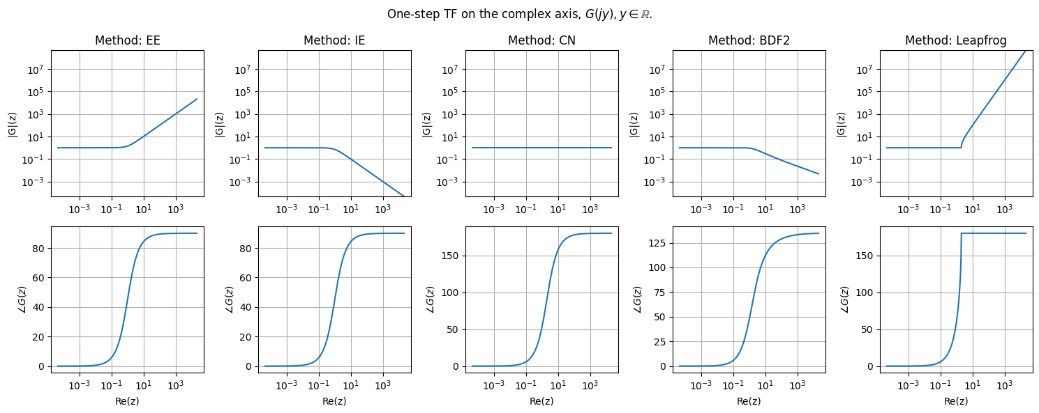
Remark. For multiple-steps methods, like BDF2 and Leapfrog, the magnitude and phase of the eigenvalue of the one-step matrix \(\mathbf{G}(z)\) is shown here.

L-stable methods. Among the methods shown here, only IE and BDF2 are L-stable, i.e. with \(|G(z \rightarrow +\infty)| \rightarrow 0\)

29.3.2.4. Dahlquist barriers - for linear multi-step methods

First Dahlquist barrier.

• A zero-stable and linear q-step multis-tep method has maximum order of convergence \(q+1\) if \(q\) is odd, \(q+2\) if \(q\) is even. If the method is explicit, maximum order of convergence is \(q\).

Second Dahlquist barrier.

• No explicit linear multi-step method is A-stable

• Maximum order of an (implicit) A-stable linear multi-step method is 2

• Among the A-stable multi-step methods of order 2, the trapezoidal rule has the smallest error constant

A linear multi-step method for the equation \(y'=f(t,y)\) with initial conditions \(y(t_0) = y_0\), reads

\[\sum_{j=0}^{s} a_j y_{n+j} = h \sum_{j=0}^{s} b_j f(t_{n+j}, y_{n+j})\]

If \(b_0 = 0\), the method is explicit, otherwise it’s implicit as the unknown \(y_{n+s}\) appears in both the LHS and the RHS.

A-stability. For the equation \(y' = \lambda y\), i.e. \(f(t,y) = \lambda y\), the \(Z\)-transformed integration step becomes

\[0 = \sum_{j=0}^{s} (a_j - h \lambda b_j ) \zeta^{j-s} = \rho(\zeta) - z \sigma(\zeta) = \pi(\zeta, z) \ ,\]

with \(z := h \lambda\).

For explicit methods, \(b_0 = 0\), the degree of \(\sigma(\zeta)\) is lower than the degree of \(\rho(\zeta)\)

…