Non-convex hyperbolic problems

35.11. Non-convex hyperbolic problems#

In this section, non-convex hyperbolic problems are briefly discussed using a non-linear scalar equation as a toy problem to show their characteristics. The main topic is the solution of a Riemann problem. Depending on the initial conditions, the solution of the Rieamnn problem for a non-convex hyperbolic scalar equation may involve not only simple waves (like shock or rarefaction), but also composite waves, combining both a shock and a rarefaction.

First, a numerical simulation of a Riemann problem the viscous counterpart of the hyperbolic equation is performed and the solution is discussed. Then, the solution is discussed introducing the Olenik criterion to find the physical solution.

35.11.1. Toy problem#

The non-linear scalar equation

\[\partial_t u + \partial_x F(u) = 0 \ ,\]

with flux $F(u) = u^3$ is a hyperbolic equation with non-convex flux, as

\[\begin{split}F''(u) = 6 u \left\{ \begin{aligned} > 0 && \text{for $u > 0$} \\ \le 0 && \text{for $u \le 0$} \end{aligned} \right.\end{split}\]

35.11.1.1. Numerical simulation#

The numerical simulation of two Riemann problem of the viscous counterpart of the hyperbolic equation,

\[\partial_t u + \partial_x F(u) - \partial_x ( \nu \partial_x u ) = 0 \ ,\]

is performed here with a time-explicit finite-difference method for two different initial conditions: $1)$ $(u_L, u_R) = (-1, 1)$, $2)$ $(u_L, u_R) = (1,-1)$.

Here, the value of the diffusion coefficient is choosen as $\nu = .05$ as a compromise between thickness of the “shock” and the stability requirement of the numerical method.

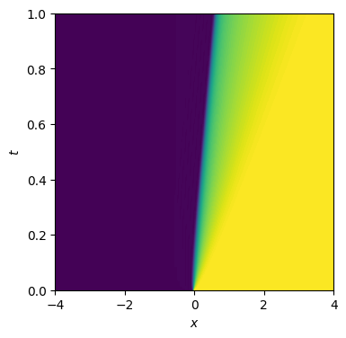
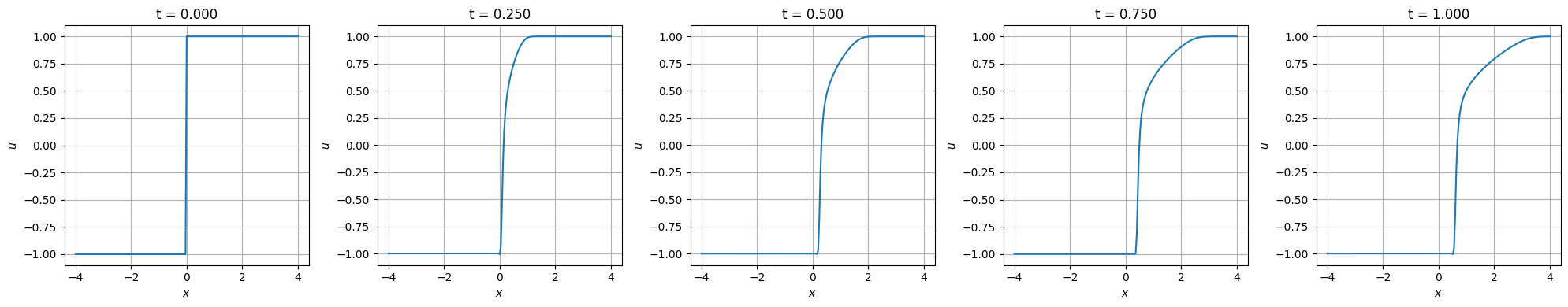
35.11.1.1.1. Simulation with $(u_L, u_R) = (-1,1)$#

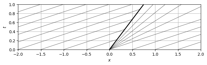
The solution is the combination of a left shock between state $u_L = -1$ and an intermediate state $u^* = \frac{1}{2}$, and a right fan between $u^*$ and $u_R = 1$.

../../_images/62f09820879672509761278e8a76e8c744cc70b0b4bd8721667cf69d4d489dd1.png

../../_images/927184ccb33f28ec505b4b577ad463e1502ad0bd744ff89ef0062b1cb57e779c.png

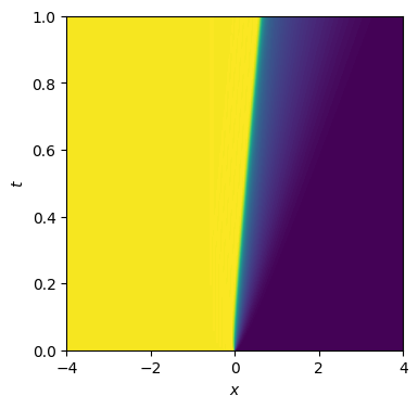
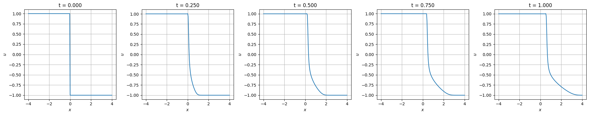
35.11.1.1.2. Simulation with $(u_L, u_R) = (1,-1)$#

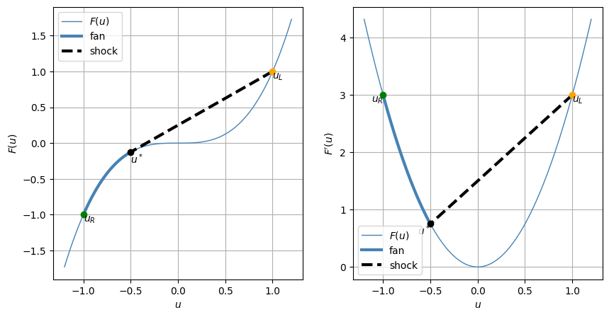
The solution is the combination of a left shock between state $u_L = 1$ and an intermediate state $u^* = \frac{1}{2}$, and a right fan between $u^*$ and $u_R = -1$.

../../_images/65f7878e97b08545f51712ca23841eba1df11ffe12d3abcacf89c43b7f787cb4.png

../../_images/4f920562eaa78bae529cf1d365558cc95051476b969341dc94a333519470b380.png

35.11.1.2. Olenik’s criterion#

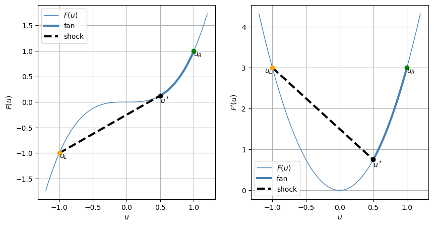
In a Riemann problem with two values $u_L$, $u_R$, with $F''(u_L) F''(u_R) < 0$ - so that non-convexity manifests itself, and assuming that $F''(u)$ changes sign only once (see the comment below for more complex flux functions -, a composite wave occurs. This composite wave is composed of a rarefaction wave and a shock wave.

The intermediate state $u^*$ is found with the condition that the speed of the shock equals the characteristic speed of the fan at the shock, i.e.

\[s(u_L, u^*) = F'(u^*) \ ,\]

or

\[\frac{F(u^*) - F(u_L)}{u^* - u_L} = F'(u^*) \ .\]

i.e. the slope $F'(u^*)$ of the tangent line at $F(u)$ in $u^*$ equals the slope of the line connecting the state $(\cdot)^*$ with $(\cdot)_L$. This condition prevents characteristic lines from originating from the shock.

An alternative formulation of Olenik’s criterion reads: for a shock to be stable, the shock speed $s$ must be the slowest possible. For $u_L > u_R$,

\[\frac{f(u) - f(u_L)}{u - u_L} \ge s(u) \ge \frac{f(u) - f(u_R)}{u-u_R} \qquad s \in [ u_L, u_R ] \ .\]

todo

With more “complex” flux functions $F(u)$ (that have several ranges of $u$-values where $F''(u)$ changes sign), how many waves in the composite wave? Show how Olenik’s criterion applies.

35.11.1.2.1. $(u_L, u_R) = (-1, 1)$#

../../_images/2e7bc7cbcedeef60b69d11a70e48e43e2c721827a1564b49aad01f8ddb1c611a.png

35.11.1.2.2. Characteristic lines in the $x-t$ plane#

../../_images/49298c4710404421e8e9130890fa19d3f528d55ac972bf3bf74cb2f9f5cef152.png

35.11.1.2.3. $(u_L, u_R) = (1, -1)$#

../../_images/94c409540621c4ccbf8bf66c74bb9d82adb00a82325c5dbe30baa8b0356af42f.png

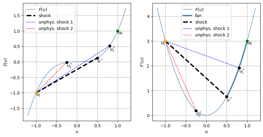
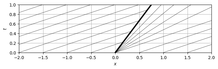
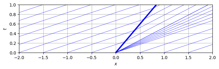
35.11.1.3. Non-physical solutions for $(u_L, u_R) = (-1, 1)$#

Show code cell source Hide code cell source

uL, uR = -1., 1.
us  = 0.5
us1 = 0.8
us2 =-0.25

fig, ax = plt.subplots(1,2, figsize=(10,5))

uv = np.linspace(-1.2, 1.2, 100)
fuv = flux(uv)
dfuv = dflux(uv)

uv_sR = np.linspace(us, uR, 100)
fuv_sR = flux(uv_sR)
dfuv_sR = dflux(uv_sR)

ax[0].plot(uv   , fuv   , lw=1., color='steelblue', label=r'$F(u)$')
ax[0].plot([uL, us], [flux(uL), flux(us)], 'k--', lw=3, label='shock')
ax[0].plot([uL, us1], [flux(uL), flux(us1)], '--', color='blue', lw=1, label='unphys. shock 1')
ax[0].plot([uL, us2], [flux(uL), flux(us2)], '--', color='red' , lw=1, label='unphys. shock 2')
ax[0].plot(uL, flux(uL), 'o', color='orange'); ax[0].text(uL, flux(uL), r'$u_L$', va='top')
ax[0].plot(uR, flux(uR), 'o', color='green' ); ax[0].text(uR, flux(uR), r'$u_R$', va='top')
ax[0].plot(us, flux(us), 'o', color='black' ); ax[0].text(us, flux(us), r'$u^*$', va='top')
ax[0].plot(us1, flux(us1), 'o', color='black' ); ax[0].text(us1, flux(us1), r'$u_1^*$', va='top')
ax[0].plot(us2, flux(us2), 'o', color='black' ); ax[0].text(us2, flux(us2), r'$u_2^*$', va='top')
ax[0].set_xlabel(r'$u$')
ax[0].set_ylabel(r'$F(u)$')
ax[0].legend()
ax[0].grid()


ax[1].plot(uv   , dfuv   , lw=1., color='steelblue', label=r'$F(u)$')
ax[1].plot(uv_sR, dfuv_sR, lw=3., color='steelblue', label=r'fan'   )
ax[1].plot([uL, us], [dflux(uL), dflux(us)], 'k--', lw=3, label='shock')
ax[1].plot([uL, us1], [dflux(uL), dflux(us1)], '--', color='blue', lw=1, label='unphys. shock 1')
ax[1].plot([uL, us2], [dflux(uL), dflux(us2)], '--', color='red' , lw=1, label='unphys. shock 2')
ax[1].plot(uL, dflux(uL), 'o', color='orange'); ax[1].text(uL, dflux(uL), r'$u_L$', va='top', ha='right')
ax[1].plot(uR, dflux(uR), 'o', color='green' ); ax[1].text(uR, dflux(uR), r'$u_R$', va='top')
ax[1].plot(us, dflux(us), 'o', color='black' ); ax[1].text(us, dflux(us), r'$u^*$', va='top')
ax[1].plot(us1, dflux(us1), 'o', color='black' ); ax[1].text(us1, dflux(us1), r'$u_1^*$', va='top')
ax[1].plot(us2, dflux(us2), 'o', color='black' ); ax[1].text(us2, dflux(us2), r'$u_2^*$', va='top')
ax[1].set_xlabel(r'$u$')
ax[1].set_ylabel(r"$F'(u)$")
ax[1].legend()
ax[1].grid()

plt.show()

../../_images/bc5d527e55e10c198275dabf9ebd66291ed7b48d8d0a767e46e0833056a5a736.png

Show code cell source Hide code cell source

#> characteristic lines in xt plane
vL = dflux(uL); thetaL = np.arctan(vL)
vR = dflux(uR); thetaR = np.arctan(vR)
vs = dflux(us); thetas = np.arctan(vs)
v1 = dflux(us1); theta1 = np.arctan(v1)
v2 = dflux(us2); theta2 = np.arctan(v2)
vs1 = ( flux(us1) - flux(uL) ) / ( us1 - uL ); thetas1 = np.arctan(vs1)
vs2 = ( flux(us2) - flux(uL) ) / ( us2 - uL ); thetas2 = np.arctan(vs2)


t_plot = 1.

#> 1. Physical solution
fig, ax = plt.subplots(1,1, figsize=(8,8))

#> Fan
n_angles = 5
for iv in range(n_angles):
    theta = thetas + iv/n_angles * (thetaR-thetas)
    vel = np.tan(theta)
    ax.plot([0, vel*t_plot], [0, t_plot], color='black', lw=0.5)

#> Shock
ax.plot([0, vs*t_plot], [0, t_plot], color='black', lw=3)

#> Uniform regions
for iv in range(10):
    dx = - iv * .5
    #> Intersection x(t) = dx + vL * t, xs(t) = vs * t
    t_int = dx / ( vs - vL )
    ax.plot([ dx, dx+vL*t_int], [0, t_int], color='black', lw=.5)

for iv in range(5):
    dx = iv * .5
    ax.plot([ dx, dx+vR*t_plot], [0, t_plot], color='black', lw=.5)

ax.set_aspect('equal')
ax.set_xlabel(r'$x$')
ax.set_ylabel(r'$t$')
ax.set_xlim(-2,2)
ax.set_ylim(0,t_plot)
ax.grid()
plt.show()

#> 2. Unphysical solution n.1
fig, ax = plt.subplots(1,1, figsize=(8,8))

#> Fan
n_angles = 5
for iv in range(n_angles):
    theta = theta1 + iv/n_angles * (thetaR-theta1)
    vel = np.tan(theta)
    ax.plot([0, vel*t_plot], [0, t_plot], color='blue', lw=0.5)

#> Shock
ax.plot([0, vs1*t_plot], [0, t_plot], color='blue', lw=3)

#> Uniform regions
for iv in range(10):
    dx = - iv * .5
    #> Intersection x(t) = dx + vL * t, xs(t) = vs * t
    t_int = dx / ( vs1 - vL )
    ax.plot([ dx, dx+vL*t_int], [0, t_int], color='blue', lw=.5)

for iv in range(5):
    dx = iv * .5
    ax.plot([ dx, dx+vR*t_plot], [0, t_plot], color='blue', lw=.5)

#> Uniform region with characteristics originating from the shock
#> Intersection x(t) = dx + v1 * t, xs(t) = vs1 * t
for iv in range(5):
    dx = - iv * .25
    t_int = dx / ( vs1 - v1 )
    ax.plot([ dx+v1*t_int, dx+v1*t_plot], [t_int, t_plot], color='blue', lw=.5)

ax.set_aspect('equal')
ax.set_xlabel(r'$x$')
ax.set_ylabel(r'$t$')
ax.set_xlim(-2,2)
ax.set_ylim(0,t_plot)
ax.grid()
plt.show()


#> 3. Unphysical solution n.2
fig, ax = plt.subplots(1,1, figsize=(8,8))

#> Fan
n_angles = 10
for iv in range(n_angles):
    theta = theta2 + iv/n_angles * (thetaR-theta2)
    vel = np.tan(theta)
    if ( vel > vs2 ):
        ax.plot([0, vel*t_plot], [0, t_plot], color='red', lw=0.5)

#> Shock
ax.plot([0, vs2*t_plot], [0, t_plot], color='red', lw=3)

#> Uniform regions
for iv in range(10):
    dx = - iv * .5
    #> Intersection x(t) = dx + vL * t, xs(t) = vs * t
    t_int = dx / ( vs2 - vL )
    ax.plot([ dx, dx+vL*t_int], [0, t_int], color='red', lw=.5)

for iv in range(5):
    dx = iv * .5
    ax.plot([ dx, dx+vR*t_plot], [0, t_plot], color='red', lw=.5)

ax.set_aspect('equal')
ax.set_xlabel(r'$x$')
ax.set_ylabel(r'$t$')
ax.set_xlim(-2,2)
ax.set_ylim(0,t_plot)
ax.grid()
plt.show()

../../_images/4f4dada3a4b1ff53ea6864f1345718fcc8d12669941012a11d0e12af7de44594.png

../../_images/20c0e74ee2e77dde5f930b328be2cbfc39bb6bfe955a967a13e5390f03cf8739.png

../../_images/08477f05fc22d95e8efba57fa7b1050027e3a6e78bd83bbc94e7db901dc4f03a.png

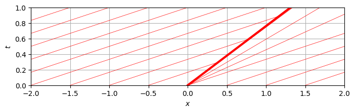
todo

The blue unphysical solution looks unphysical for the characteristic lines orginating from the shock. But why is the red solution unphysical?
Discussion about local stability
Discussion with local production of entropy $\Sigma(u) = s(u) [ \eta (u) ] - [ q(u) ]$, and extreme points at the physical solution $u^*$? $\Sigma'(u^*) = 0$?

Non-convex hyperbolic problems

Contents

35.11. Non-convex hyperbolic problems#

35.11.1. Toy problem#

35.11.1.1. Numerical simulation#

35.11.1.1.1. Simulation with \((u_L, u_R) = (-1,1)\)#

35.11.1.1.2. Simulation with \((u_L, u_R) = (1,-1)\)#

35.11.1.2. Olenik’s criterion#

35.11.1.2.1. \((u_L, u_R) = (-1, 1)\)#

35.11.1.2.2. Characteristic lines in the \(x-t\) plane#

35.11.1.2.3. \((u_L, u_R) = (1, -1)\)#

35.11.1.3. Non-physical solutions for \((u_L, u_R) = (-1, 1)\)#