58.1. 1-dimensional Poisson equation#
58.1.1. Integral form of the problem#
The integral form of a Poisson problem reads, for every \(V \in \Omega\),
supplied with proper boundary conditions. As an example,
Dirichlet boundary conditions: \(u(\overline{x}) = \overline{u}\)
Neumann boundary conditions: \(\nu \hat{\mathbf{n}} \cdot \nabla u(\overline{x}) = \overline{q}\)
Robin boundary conditions: \(a u(\overline{x}) + b u'(\overline{x}) = c\)
The multi-dimensional set may be useful also for 1-dimensional domains, to avoid confusions with signs
58.1.2. Domain, volume forcing and boundary conditions#
import numpy as np
import scipy as sp

import matplotlib.pyplot as plt

#> Domain
a, b = 0, 1
l = b - a

#> Physical properties
nu = .01                       # Diffusion coefficient
f = 1.

#> Discretization
nel = 10            # n.of elements
nnodes = nel + 1    # n.of nodes
nvol = nnodes       # n.finite volumes (node-centered FVM)

#> Dirichlet boundaries
i_dir = np.array([ 0, nvol-1])   # Global idx of nodes on Dirichlet boundaries
u_dir = np.array([ .0, .0 ])   # Value of the solution at nodes on Dir. boundaries

#> Volume forcing contribution
f_nodal = np.ones(nel+1) * f   # Nodal values f(x_i) of volume forcing, here uniform f(x) = f

#> Node centered FVM
rr_n = np.linspace(a,b, nel+1)       # node coordinates (center of the node-centered FVs)
rr_i = .5 * ( rr_n[:-1] + rr_n[1:] ) # coords of the inner cell interface
rr_b = np.array([ 2*rr_n[0]-rr_n[1], 2*rr_n[-1]-rr_n[-2] ])  # coords of the boundaries

vols = np.array(
     [ np.abs(rr_i[0]-rr_n[0]) ] + \
       list( np.abs(rr_i[1:] - rr_i[:-1]) ) + \
     [ np.abs(rr_i[-1]-rr_n[-1]) ]
)

ni = len(rr_i)
nb = len(rr_b)

#> Interface-volume connectivity (ni, 2) (normal dir: first element -> second element)
iee = np.array([ [i, i+1] for i in np.arange(ni) ])
#> Boundary-volume connectivity (nb) (convention, normal dir: elem -> outside)
bee = np.array([0, nvol-1])
58.1.3. Discrete matheamtical problem#
#> Evaluating boundary contributions
# Here assmbling a stiffness matrix. In many FVM applications, there's explicit time
# dependence and explicit time integration schemes are used, so there's no need to
# assemble any matrix while the algorithm just rely on accumulation of flux contributions
# -> Add a link to a script implementing time-dependent "solver" for FVM, e.g. hyperbolic problems

i_flux, j_flux, e_flux = [], [], []

#> Loop over internal interface
# accumulating and keep changing the dimension! May be very inefficient and slow
for i in np.arange(ni):
    flux_u = nu / np.abs( rr_n[ iee[i,1] ] - rr_n[ iee[i,0] ] )
    i_flux += [ iee[i,0], iee[i,0], iee[i,1], iee[i,1] ]
    j_flux += [ iee[i,0], iee[i,1], iee[i,0], iee[i,1] ]
    e_flux += [ -flux_u, flux_u, flux_u, -flux_u ]

e_flux = -np.array(e_flux)

K = sp.sparse.coo_array((e_flux, (i_flux, j_flux)),)

#> Volume forcing
F = vols * f

#> Loop over boundary surfaces
# ...
# - Neumann: add a forcing term for finite volumes with sides on Neumann boundaries
# - Dirichlet: prescribe node value (e.g. 1) matrix slicing, 2) augmented system,...)
# - Robin: add a forcing term depending on the unknown value of the function -> modify K matrix

# ...
58.1.4. Applying essential boundary conditions#
The discrete counterpart of the continuous problem is a linear system that can be formally written as \(\mathbf{A} \mathbf{u} = \mathbf{f}\). So far, the essential boundary conditions on Dirichlet boundary \(S_D\) have not been prescribed yet. Essential boundary conditions can be prescribed in (at least) two ways: 1) slicing the linear system; 2) augmenting the linear system.
Method 1. Slicing the linear system. The set of nodes \((\cdot)_d\) lying on Dirichlet boundaries can be distinguished from all the remaining nodes \((\cdot)_u\), and the linear system sliced accordingly
On \(u\)-nodes, forcing \(\mathbf{f}_u\) is known, while the value of the function \(u(\mathbf{x})\) is unknown, and thus \(\mathbf{u}_n\) is unknown; on the other hand, on \(d\)-nodes the value of the function \(u(\mathbf{x})\) is known, and so \(\mathbf{u}_d = \mathbf{u}_D\) is known, while the forcing \(\mathbf{f}_d\) is not known (as it contains both a volume contribution and a “boundary contribution” required to prescribe essential boundary conditions, as it will be more clear later, hopefully).
After slicing, the problem is solved first finding \(\mathbf{u}_u\) and then retrieving the value of \(\mathbf{f}_d\),
Method 2. Augmenting the linear system. The linear system is augmented, a) explicityl adding equations \(\mathbf{u}_d = \mathbf{u}_D\) for the essential boudary conditions, and splitting the forcing contribution on Dirichlet nodes as the sum of a known volume contribution and an unknown boundary contribution,
Moving all the unkowns on the LHS, the augmented linear system reads
The (arbitrary) choice of the sign in the last block of equations (the ones prescribing the value of the unknown function on Dirichlet boundary) is usually chosen to preserve the symmetry of the original problem, if any.
todo Discuss the reason why the system becomes determinate, after the application of the essential b.c.s
58.1.4.1. Slicing the linear system#
Slice the linear system to prescribe the essential boundary conditions, solve the linear system, retrieve and plot the results.
#> Apply essential boundary conditions, solve the linear system and retrieve the solution
#> Method 1. Slicing matrices
# K u = f
# [ Kuu Kud ] [ uu ] = [ fu ]
# [ Kdu Kdd ] [ ud ] [ fd ]
# with known: ud, fu; unknown: uu, fd found solving the problem
# Kuu * uu = fuu - Kud * ud -> uu = ...
# fd = Kdu * uu + Kdd * ud
iD = i_dir.copy()
iU = np.array(list(set(np.arange(nnodes)) - set(iD)))
ud = u_dir.copy()
print(iD)
print(iU)
#> Slice stiffness matrix
Kuu = (K.tocsc()[:,iU]).tocsr()[iU,:]
Kud = (K.tocsc()[:,iD]).tocsr()[iU,:]
Kdu = (K.tocsc()[:,iU]).tocsr()[iD,:]
Kdd = (K.tocsc()[:,iD]).tocsr()[iD,:]
#> Slice forcing
fu = F[iU]
#> Solve the linear system
uu = sp.sparse.linalg.spsolve(Kuu, fu - Kud @ ud )
fd = Kdu @ uu + Kdd @ ud
#> Re-assemble the solution
u = np.zeros(nnodes); u[iU] = uu; u[iD] = ud
f = np.zeros(nnodes); f[iU] = fu; f[iD] = fd
# print("uu: \n", uu)
# print("Fd: \n", fd)
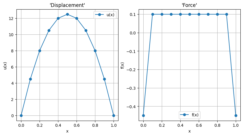
#> Plot some results
fig, ax = plt.subplots(1,2, figsize=(10, 5))
ax[0].plot(rr_n, u, '-o', label='u(x)')
ax[0].legend()
ax[0].grid()
ax[0].set_title('\'Displacement\'')
ax[0].set_xlabel('x')
ax[0].set_ylabel('u(x)')
ax[1].plot(rr_n, f, '-o', label='f(x)')
ax[1].legend()
ax[1].grid()
ax[1].set_title('\'Force\'')
ax[1].set_xlabel('x')
ax[1].set_ylabel('f(x)')
[ 0 10]
[1 2 3 4 5 6 7 8 9]
Text(0, 0.5, 'f(x)')
58.1.4.2. Augmenting the linear system#
Augmenting the linear system to prescribe the essential boundary conditions, solve the linear system, retrieve and plot the results.
todo
#> Method 2. Augmented system
# ...
Some comments and todos.
Convergence analysis. It’s possible to evaluate both convergence with the dimension of the elements and/or the degree of the polynomial base functions. The exact solution can be easily computed analytically via direct integration for simple distribution of load \(f(x)\), and uniform \(\nu\)
Result discussion. “Force” contribution on Dirichlet boundary conditions involves both the node contribution to distributed load and the “constraint reaction”. As an example, with a domain of size \(\ell\) and uniform force distribution \(f\), with \(u(0) = u(\ell) = 0\), by symmetry and global equilibrium the force at boundaries are \(-\frac{1}{2} q \ell = - \frac{1}{2}\). With the modelling choices done, the contribution of the uniform distributed load on an element on any of its nodes is \(\frac{1}{2} q \ell_i = \frac{1}{2} q \frac{\ell}{n_{el}}\). Here with \(n_{el} = 20\), this elementary contribution is \(\frac{1}{40} = .025\): thus, the nodal contribution of internal nodes is twice (contribution from two neighboring elements) this value \(.05\), and the force on each Dirichlet boundary is \(-\frac{1}{2} + \frac{1}{40} = - 0.475\).
Try to set different values of Dirichlet boundary conditions, u_dir