58.4.4. 1-dimensional Euler equations for Perfect Ideal Gas on moving mesh (ALE)#
Integral equations for general domain \(v_t\). Starting from the balance equation for a control volume \(V\) at rest,
\[\frac{d}{dt}\int_{V} \mathbf{u} + \oint_{\partial V} \mathbf{F}(\mathbf{u}) \cdot \hat{\mathbf{n}} = \int_{V} \mathbf{s} \ ,\]
using Reynolds’ transport theorem, the balance equation for an arbitrary volume \(v_t\) follows
\[\frac{d}{dt}\int_{v_t} \mathbf{u} - \oint_{\partial v_t} \mathbf{u} \mathbf{v}_b \cdot \hat{\mathbf{n}} + \oint_{\partial v_t} \mathbf{F}(\mathbf{u}) \cdot \hat{\mathbf{n}} = \int_{v_t} \mathbf{s} \ ,\]
or collecting all the boundary terms
\[\frac{d}{dt}\int_{v_t} \mathbf{u} + \oint_{\partial v_t} \left[ \mathbf{F}(\mathbf{u}) - \mathbf{u} \mathbf{v}_b \right] \cdot \hat{\mathbf{n}} = \int_{v_t} \mathbf{s} \ .\]
Explicit Euler scheme
\[( \mathbf{u}_i^{n+1} V_i^{n+1} ) = ( \mathbf{u}_i^{n} V_i^{n} ) - \Delta t \sum_{j \in B_i} \mathbf{F}_j^n \ ,\]
Roe flux …
Boundary conditions
58.4.4.1. Useful classes for numerical methods#
58.4.4.1.1. Basic libraries#
Show code cell source
import numpy as np
import matplotlib.pyplot as plt
58.4.4.1.2. Parent class#
\(\texttt{HyperbolicSystem1d()}\) class with common functions (or just their templates) required to implement a finite volume method solver.
Show code cell source
class HyperbolicSystem1d():
    """
    Analytical quantities of a Hyperbolic linear system in a 1-dimensional domain
    """
    def __init(self, **params):
        pass
    def flux(self,):
        """ Analytical flux, f """
        pass
    def A(self,):
        """ Advection matrix, A """
        pass
    def s(self,):
        """ Eigenvalues of matrix, s """
        pass
    def R(self,):
        """ Matrix of right eigenvectors, R """
        pass
    def L(self,):
        """ Matrix of left eigenvectors, L=inv(R) """
        pass
    def spectrum(self,):
        """ Spectrum of matrix A() """
        return self.s(), self.R(), self.L()

    def absA(self, u):
        """ A = R * S * L, |A| = R * |S| * L """
        return self.R(u) @ np.diag(np.abs(self.s(u))) @ self.L(u)

    def roe_intermediate_state(self,):
        """ Roe intermediate state for Roe linearization """
        pass
58.4.4.1.3. Euler equations for perfect ideal gas class#
Show code cell source
class Euler1dPIG(HyperbolicSystem1d):
    """
    Analytical quantities of a Hyperbolic linear system in a 1-dimensional domain
    Physical quantities:
    - conservative: (rho, m, Et)
    - physical/convective (rho, u, e) or (rho, u, s)
    Parameters:
    - gamma: cp/cv ratio

    PIG (Perfect Ideal Gas)
    gamma = cp / cv  --> cv =     1 / ( gamma - 1 ) * R
    cp - cv = R      --> cp = gamma / ( gamma - 1 ) * R
    p = rho * R * T = rho * R/cv e = (gamma-1) * rho * e = (gamma-1) * E
    e = cv * T
    """
    def __init__(self, gamma=5./3., name=""):
        """  """
        # Speed of sound, a, and pressure, p,  are functions of the TD state
        # ...add functions fun_a(...), fun_p(...)
        # - which physical variables?
        # - equations of state for different fluids (PIG, VdW,...)
        self.gamma = gamma
        self.gamma_1 = self.gamma - 1
        self.name = name

    def fun_p(self, u):
        """
        Pressure as a function of conservative variables
        p = rho R T = rho R/cv e = (gamma-1) rho e = (gamma-1) ( Et - .5* m^2/rho)
        """
        return self.gamma_1 * ( u[2] - .5 * u[1]**2 / u[0] )

    def phys_from_cons(self, u):
        """
        rho = rho
        u   = m / rho
        p   = (gamma-1) * E
            = (gamma-1) * ( Et - .5 * rho * u^2 )
            = (gamma-1) * ( Et - .5 * m^2 / rho )
        """
        return np.array([ u[0], u[1]/u[0], self.fun_p(u) ])

    def cons_from_phys(self, p):
        """
        rho = rho
        m   = rho * u
        Et  = rho * ( e + .5 * u^2 )
            = E + .5 * rho * u^2
            = p / ( gamma - 1 ) + .5 * rho * u^2
        """
        Et = p[2]/self.gamma_1 + .5 * p[0] * p[1]**2
        return np.array([ p[0], p[0]*p[1], Et])

    def flux(self, u):
        """ Numerical flux
        u: conservative variables (rho, m, Et)
        F = ( m, rho*u^2+p(...), u*(Et+p(...)) )
        """
        vel = u[1]/u[0]
        p = self.fun_p(u)
        return np.array([ u[1], u[0]*vel**2+p, vel*(u[2]+p) ])

    def A(self, u):
        """
        Convection matrix, A; input: conservative variables
        A = [[            0,        1,         0 ],
             [    u^2+p_rho,   2u+p_m,      p_Et ],
             [-u*ht+u*p_rho, ht+u*p_m, u*(1+p_Et)]]
        """
        vel = u[1]/u[0]
        p = self.fun_p(u)
        ht = ( u[2] + p ) / u[0]
        p_rho = .5 * self.gamma_1 * vel**2
        p_m   = - self.gamma_1 * vel
        p_Et  =   self.gamma_1
        return np.array(
            [[ .0, 1.,.0 ],
             [ -vel**2+p_rho, 2*vel+p_m, p_Et ],
             [  vel*(-ht+p_rho), ht+vel*p_m, vel*(1+p_Et) ]])

    def s(self, u):
        """
        Eigenvalues of A; input: conservative variables
        s = [u-a, u, u+a]
        """
        vel = u[1]/u[0]
        p = self.fun_p(u)
        # Speed of sound, a^2 = gamma R T = gamma p / rho
        a = np.sqrt(self.gamma * self.fun_p(u)/u[0])
        return np.array([vel-a, vel, vel+a])

    def R(self, u):
        """
        Right eigenvectors of A; input: conservative variables
        R = ...
        """
        vel = u[1]/u[0]
        p = self.fun_p(u)
        # Speed of sound, a^2 = gamma R T = gamma p / rho
        a = np.sqrt(self.gamma * self.fun_p(u)/u[0])
        ht = ( u[2] + p ) / u[0]
        p_rho = .5 * self.gamma_1 * vel**2
        p_m   = - self.gamma_1 * vel
        p_Et  =   self.gamma_1

        return np.array([
            [1, vel-a, ht-vel*a],
            [1, vel  , vel**2-p_rho/p_Et],
            [1, vel+a, ht+vel*a]]).T

    def L(self, u):
        """
        Left eigenvectors of A; input: conservative variables
        L = ...
        """
        vel = u[1]/u[0]
        p = self.fun_p(u)
        # Speed of sound, a^2 = gamma R T = gamma p / rho
        a = np.sqrt(self.gamma * self.fun_p(u)/u[0])
        ht = ( u[2] + p ) / u[0]
        p_rho = .5 * self.gamma_1 * vel**2
        p_m   = - self.gamma_1 * vel
        p_Et  =   self.gamma_1

        return np.array([
            [ p_rho + vel*a ,   p_m - a  ,   p_Et ],
            [-2*(p_rho-a**2),-2*p_m      ,-2*p_Et ],
            [ p_rho - vel*a ,   p_m + a  ,   p_Et ]
            ]) / ( 2. * a**2 )

    def spectrum(self, u):
        """ Spectrum of matrix A; input: conservative variables """
        return self.s(u), self.R(u), self.L(u)

    def roe_intermediate_state(self, u_0, u_1):
        """
        For p-sys:
          rho_roe = ANY! = ... CHOOSE ONE: average = 0.5*(rho_0+rho_1)
          vel_roe = (sqrt(rho_0)*vel_0+sqrt(rho_1)*vel_1)/(sqrt(rho_0)+sqrt(rho_1))
          - convective/physical: (rho, vel) = ( rho_roe, vel_roe )
          - conservatvie       : (rho, mom) = ( rho_roe, rho_roe*vel_roe)
          F_roe(u) ~ dFdu * du ~ A(u_roe(u0,u1)) * (u_1 - u_0)
        """
        #> Density (for a PIG, it's arbitrary once consistency is provided)
        rho_roe = np.sqrt(u_0[0]*u_1[0])  #.5*(u_0[0]+u_1[0])

        vel_0, vel_1 = u_0[1]/u_0[0], u_1[1]/u_1[0]
        p_0, p_1 = self.fun_p(u_0), self.fun_p(u_1)
        ht_0, ht_1 = ( u_0[2] + p_0 ) / u_0[0],  ( u_1[2] + p_1 ) / u_1[0]

        #> Velocity and total enthalpy (Roe linearization)
        vel_roe = (vel_0*np.sqrt(u_0[0])+vel_1*np.sqrt(u_1[0])) / \
                  (np.sqrt(u_0[0])+np.sqrt(u_1[0]))
        ht_roe  = ( ht_0*np.sqrt(u_0[0])+ ht_1*np.sqrt(u_1[0])) / \
                  (np.sqrt(u_0[0])+np.sqrt(u_1[0]))

        #> Enthalpy and pressure (PIG)
        h_roe = ht_roe - .5 * vel_roe**2
        # p = rho R T = rho R/cP h = (gamma-1)/gamma * rho * h
        p_roe = self.gamma_1/self.gamma * rho_roe * h_roe

        #> Momentum and total energy
        m_roe = rho_roe * vel_roe
        Et_roe = rho_roe * ht_roe - p_roe

        return np.array([rho_roe, m_roe, Et_roe])

    def absA_entropy_fix(self, u, delta=.1, vel=.0):
        """  """
        #> Eigenvalues s1 = u-a, s2 = u, s3 = u+a
        eigvals = self.s(u) - vel
        #> Speed of sound a = .5 * ( s3 - s1 )
        a = .5 * ( np.max(eigvals) - np.min(eigvals) )
        #> Entropy fix
        entropy_evals = np.abs(eigvals)
        entropy_evals[entropy_evals < delta*a] = \
            .5 * entropy_evals[entropy_evals < delta*a]**2 / ( delta * a ) + .5 * ( delta * a )

        return  self.R(u) @ np.diag(entropy_evals) @ self.L(u)

    def roe_flux(self, u_0, u_1, delta=.1, vel=.0, debug=False):
        """  """

        u_roe = self.roe_intermediate_state(u_0, u_1)

        if ( debug == True ):
            print("u_roe: ", u_roe)
            print("vel: ", vel)
            print("f0: ", self.flux(u_0))
            print("vel*u0 :", vel * u_0)
            print("f1: ", self.flux(u_1))
            print("vel*u1 :", vel * u_1)

        return .5 * (self.flux(u_1) - vel*u_1 + self.flux(u_0) - vel*u_0 - \
                     self.absA_entropy_fix(u_roe, delta=delta, vel=vel) @ ( u_1 - u_0 ) )

    def flux_at_boundary(self, boundary, u, vel=.0, debug=False):
        """
        boundary: boundary condition dict
        u: conservative variables (rho, m, Et) at boundary cell
        """

        if ( boundary["type"] == "wall" ):
            #> State in the ghost cell
            u_boundary = u.copy();
            u_boundary[1] =-u[1] + 2. * u[0] * vel                     # momentum
            u_boundary[2] = u[2] + 2. * u[0] * vel**2 - 2 * u[1] * vel # total energy

            if ( boundary["nor"] < 0 ):
                flux = self.roe_flux(u_boundary, u, vel=vel, debug=debug)
            else:
                flux = self.roe_flux(u, u_boundary, vel=vel, debug=debug)

            if ( debug == True ):
                print("> Boundary, nor:", boundary["nor"])
                print("u: ", u)
                print("u_boundary: ", u_boundary)
                print("flux: ", flux)
                print()

            return flux

        elif ( boundary["type"] == "inflow" or boundary["type"] == "outflow" ):

            delta_v = self.L(u) @ ( self.cons_from_phys(boundary["phys_ext"]) - u )
            eigval = self.s(u) - vel
            delta_v[ eigval*boundary["nor"] > 0 ] = .0
            u_flux = u + self.R(u) @ delta_v

            return self.flux(u_flux) - vel * u_flux
58.4.4.1.4. Time dependent mesh#
Time dependent mesh class, producing a mesh with uniform spacing, given the law of motion of the extreme points of the domain.
Show code cell source
class TimeDependentMesh():
    def __init__(self, ne, dt, fun_x0 = lambda t: .0, fun_x1 = lambda t: 1., t0 = .0):
        """  """
        #> Number of elements
        self.ne = ne
        self.fun_x0 = fun_x0
        self.fun_x1 = fun_x1
        self.dt = dt             # maybe it could be updated in variable-step algorithms

        #> Initialize domain
        self.update_domain(t0)

    def update_domain(self, t):
        """
        t: t old
        """

        #> Position of the interfaces (uniform mesh) at time t[n]
        self.xi = np.linspace(self.fun_x0(t), self.fun_x1(t), self.ne+1)

        #> Position of the interfaces (uniform mesh) at time t[n+1]
        self.xi_p1 = np.linspace(self.fun_x0(t+self.dt), self.fun_x1(t+self.dt), self.ne+1)

        #> Velocity of the interfaces
        self.vi = ( self.xi_p1 - self.xi ) / self.dt

        #> Cell volumes
        self.dx = self.xi[1:] - self.xi[:-1]
        self.dx_p1 = self.xi_p1[1:] - self.xi_p1[:-1]
58.4.4.2. Numerical simulation#
58.4.4.2.1. System of equations#
Initialized the system of equations to be solved
Show code cell source
# Number of unknown fields, nu
#> P-system, Shallow Water
#  - conservative       : u = (rho, mom)
#  - physical/convective: p = (rho, vel), with mom = rho*vel
#> Euler
#  - conservative       : u = (rho, mom, Et)
#  - physical/convective: p = (rho, vel, e) or = (rho, vel, s), with mom = rho*vel

gamma = 5. / 3.

#> Parameters and initialization of the system
# S = Psys1d(a=1);  nu = 2
# S = ShallowWater1d(g=1);  nu = 2
# S = Psys1dLinearized(a=1);  nu = 2
S = Euler1dPIG(gamma=gamma);  nu = 3
58.4.4.2.2. Domain#
Show code cell source
#> Parameters
ne = 50
dt = .0025

fun_x0 = lambda t: -.3 * t + 0. # -(t/0.1)**2
fun_x1 = lambda t:  .0 * t + 1. # -(t/0.1)**2

mesh = TimeDependentMesh(ne=ne, dt=dt, fun_x0=fun_x0, fun_x1=fun_x1)
xc = .5 * ( mesh.xi[:-1] + mesh.xi[1:] )
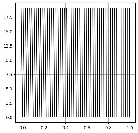
58.4.4.2.2.1. VV of the moving mesh#
Show code cell source
#> Quick check and validation of the moving mesh

it = 0

X, T = [], []

while it < 20:

    mesh.update_domain(it*mesh.dt)
    X.append(mesh.xi)
    T.append(it)

    it += 1

X = np.array(X)

fig, ax = plt.subplots(1,1, figsize=(5,5))
ax.plot(X, T, color="black")
ax.grid()
plt.show()
58.4.4.2.3. Boundary conditions#
Show code cell source
#> Boundary conditions

boundary_0 = {  # left boundary
    "type": "wall",
    "nor" : -1.
}
# boundary_1 = {  # right boundary
#     "type": "wall",
#     "nor" : 1.
# }
#> Inflow and outflow bcs are characteristic-based bcs, with the same implementation.
# They're essentially the same
# boundary_0 = {  # left boundary
#     "type": "inflow",
#     "phys_ext": np.array([2., .0, 2.]),   # rho_ext, u_ext, p_ext
#     "nor": -1.                             # nx
# }
boundary_1 = {  # right boundary
    "type": "outflow",
    "phys_ext": np.array([1., .0, 1.]),    # rho_ext, u_ext, p_ext
    "nor": 1.                              # nx
}
58.4.4.2.4. Initial conditions#
Show code cell source
#> Initial conditions, in physical variables

# #> Initial condition 0: uniform
# rhoL, rhoR = 1.0, 1.0
# velL, velR = 0.0, 0.0
# pL  , pR   = 1., 1.

#> Initial condition 1: u=0, T uniform, pL != pR
rhoL, rhoR = 1., 1.
velL, velR = 0., 0.
pL  , pR   = 1., 1.

rhoL, momL, EtL = S.cons_from_phys(np.array([rhoL, velL, pL]))
rhoR, momR, EtR = S.cons_from_phys(np.array([rhoR, velR, pR]))

#> Write initial conditions into uc0 array
uc0 = np.zeros((nu,ne))
uc0[0,:] = np.where( xc<.5, rhoL, rhoR )
uc0[1,:] = np.where( xc<.5, momL, momR )
uc0[2,:] = np.where( xc<.5, EtL , EtR  )
58.4.4.2.5. Simulation parameters#
Show code cell source
#> Time
t0, t1, dt = 0., 2.5, dt # 25
nt = int((t1-t0)/dt)+1
tv = np.arange(nt)*dt

#> Numerical schemes
#> Time integration
time_integration = 'ee'       # ...
numerical_flux   = 'roe'      # ...

#> Time loop
uuc = np.zeros((nt, nu, ne))    # Array to store solution, for small dimensional pbs
uc = uc0.copy()
uVc = uc * mesh.dx[:,np.newaxis].T
uuc[0,:,:] = uc
58.4.4.2.6. Time loop#
Show code cell source
#> Time loop
it = 0

X, T = [], []

while it < nt-1:

    t = tv[it]

    # print();  print(f"Time: {t}");  print(f"State:\n{uc}")
    mesh.update_domain(t)

    #> Evaluate fluxes at internal boundaries
    if numerical_flux == 'roe':
        flux = np.array([ S.roe_flux(uc[:,ia], uc[:,ia+1], vel=mesh.vi[ia+1]) for ia in range(ne-1) ]).T

    #> Flux at boundaries - Treat boundary conditions
    flux_0 = S.flux_at_boundary(boundary_0, uc[:, 0], vel=mesh.vi[ 0], debug=False)
    flux_1 = S.flux_at_boundary(boundary_1, uc[:,-1], vel=mesh.vi[-1], debug=False)

    # stop

    # flux = np.append(np.append(flux_0, flux), flux_1)
    flux = np.concatenate((flux_0[:,np.newaxis], flux, flux_1[:, np.newaxis]), axis=1)

    #> Time integration
    if time_integration == 'ee':
        dt = tv[it+1] - tv[it]
        # source = np.zeros((nu,ne))
        # uc += ( flux[:,:-1] - flux[:,1:] ) * dt / dx
        uVc += ( flux[:,:-1] - flux[:,1:] ) * dt
        uc = uVc / mesh.dx_p1[:,np.newaxis].T

    it += 1                   # Updating counter
    uuc[it,:,:] = uc.copy()   # Storing results
    X.append(mesh.xi)
    T.append(t*np.ones(ne))

X.append(mesh.xi_p1)
T.append((t+dt)*np.ones(ne))

X = np.array(X)
T = np.array(T)

Xc = .5 * ( X[:,:-1] + X[:,1:] )  # Cell centers
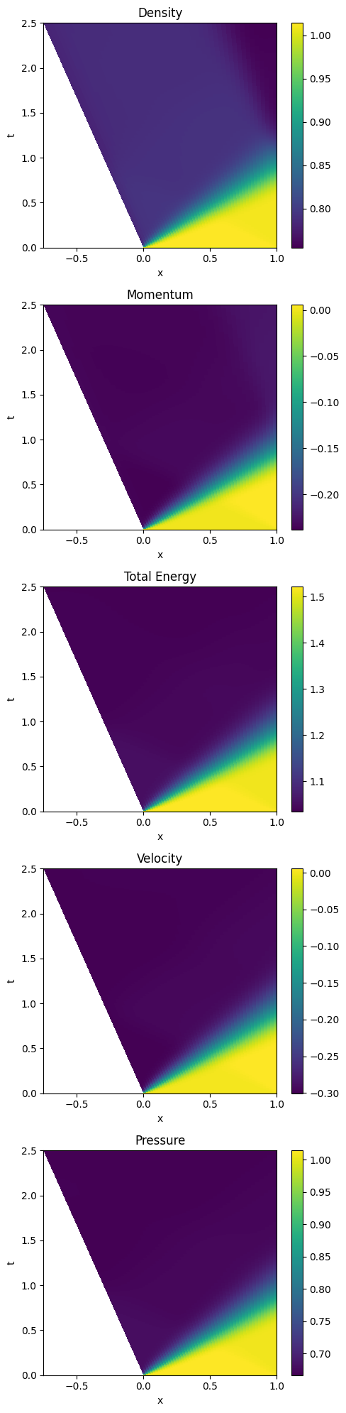
58.4.4.2.7. Post-processing#
Show code cell source
fig, ax = plt.subplots(5,1, figsize=(5,20))

iax = 0
m0 = ax[iax].pcolormesh(Xc, T, uuc[:,0,:])
# ax[iax].imshow(uuc[:,0,:], aspect="auto")
# ax[0].set_colorbar()
ax[iax].set_xlabel('x')
ax[iax].set_ylabel('t')
ax[iax].set_title('Density')
fig.colorbar(m0, ax=ax[iax])

iax = 1
m0 = ax[iax].pcolormesh(Xc, T, uuc[:,1,:])
# ax[0].set_colorbar()
ax[iax].set_xlabel('x')
ax[iax].set_ylabel('t')
ax[iax].set_title('Momentum')
fig.colorbar(m0, ax=ax[iax])

iax = 2
m0 = ax[iax].pcolormesh(Xc, T, uuc[:,2,:])
# ax[0].set_colorbar()
ax[2].set_xlabel('x')
ax[iax].set_ylabel('t')
ax[iax].set_title('Total Energy')
fig.colorbar(m0, ax=ax[iax])

iax = 3
m0 = ax[iax].pcolormesh(Xc, T, uuc[:,1,:]/uuc[:,0,:])
# ax[0].set_colorbar()
ax[iax].set_xlabel('x')
ax[iax].set_ylabel('t')
ax[iax].set_title('Velocity')
fig.colorbar(m0, ax=ax[iax])

# pressure
# p = (gamma-1) * ( Et - .5 * m^2 / rho )
iax = 4
m0 = ax[iax].pcolormesh(Xc, T, S.gamma_1 * (uuc[:,2,:]-.5*uuc[:,1,:]**2/uuc[:,0,:]))
# ax[0].set_colorbar()
ax[iax].set_xlabel('x')
ax[iax].set_ylabel('t')
ax[iax].set_title('Pressure')
fig.colorbar(m0, ax=ax[iax])

plt.tight_layout()
/tmp/ipykernel_81394/54342096.py:4: UserWarning: The input coordinates to pcolormesh are interpreted as cell centers, but are not monotonically increasing or decreasing. This may lead to incorrectly calculated cell edges, in which case, please supply explicit cell edges to pcolormesh.
  m0 = ax[iax].pcolormesh(Xc, T, uuc[:,0,:])
/tmp/ipykernel_81394/54342096.py:13: UserWarning: The input coordinates to pcolormesh are interpreted as cell centers, but are not monotonically increasing or decreasing. This may lead to incorrectly calculated cell edges, in which case, please supply explicit cell edges to pcolormesh.
  m0 = ax[iax].pcolormesh(Xc, T, uuc[:,1,:])
/tmp/ipykernel_81394/54342096.py:21: UserWarning: The input coordinates to pcolormesh are interpreted as cell centers, but are not monotonically increasing or decreasing. This may lead to incorrectly calculated cell edges, in which case, please supply explicit cell edges to pcolormesh.
  m0 = ax[iax].pcolormesh(Xc, T, uuc[:,2,:])
/tmp/ipykernel_81394/54342096.py:29: UserWarning: The input coordinates to pcolormesh are interpreted as cell centers, but are not monotonically increasing or decreasing. This may lead to incorrectly calculated cell edges, in which case, please supply explicit cell edges to pcolormesh.
  m0 = ax[iax].pcolormesh(Xc, T, uuc[:,1,:]/uuc[:,0,:])
/tmp/ipykernel_81394/54342096.py:39: UserWarning: The input coordinates to pcolormesh are interpreted as cell centers, but are not monotonically increasing or decreasing. This may lead to incorrectly calculated cell edges, in which case, please supply explicit cell edges to pcolormesh.
  m0 = ax[iax].pcolormesh(Xc, T, S.gamma_1 * (uuc[:,2,:]-.5*uuc[:,1,:]**2/uuc[:,0,:]))
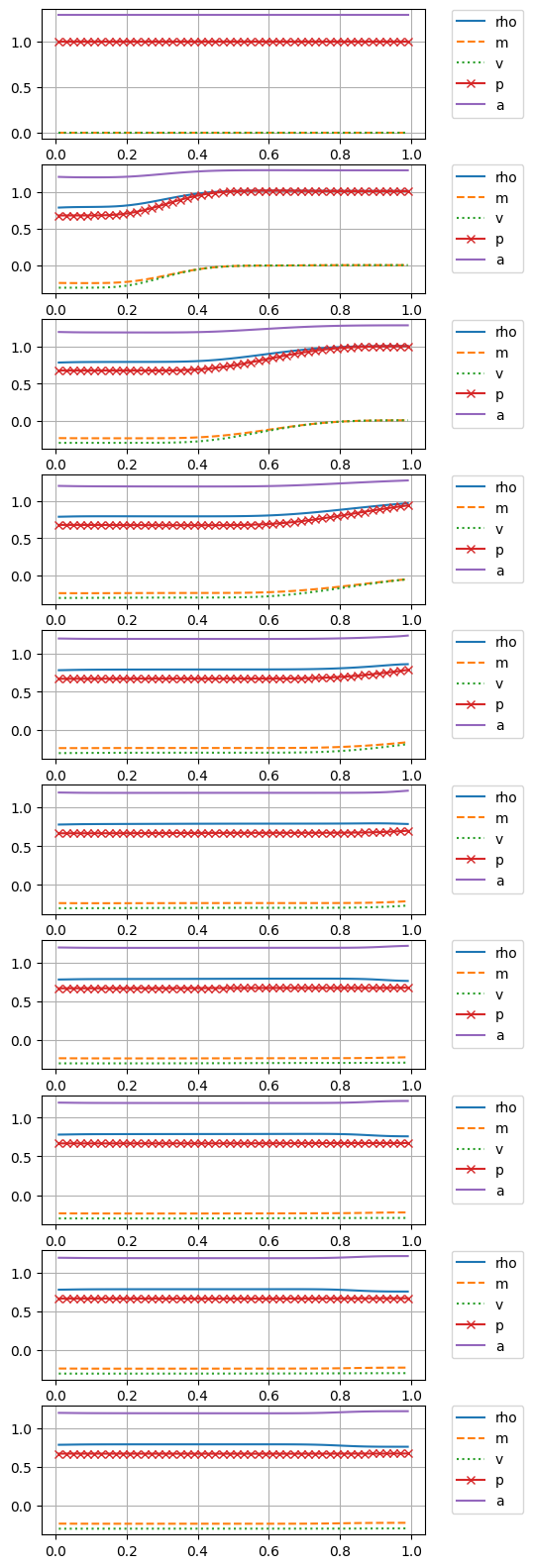
Show code cell source
n_plots = 10
i_dt = int(np.floor(nt/n_plots))

fig, ax = plt.subplots(n_plots, figsize=(5,20))
for i in range(n_plots):
    p = S.gamma_1 * (uuc[i_dt*i,2,:]-.5*uuc[i_dt*i,1,:]**2/uuc[i_dt*i,0,:])
    ax[i].plot(xc,uuc[i_dt*i,0,:], '-', label="rho")
    ax[i].plot(xc,uuc[i_dt*i,1,:], '--', label="m")
    # ax[i].plot(xc,uuc[i_dt*i,2,:], label='Et')
    ax[i].plot(xc,uuc[i_dt*i,1,:]/uuc[i_dt*i,0,:], ':', label="v")
    ax[i].plot(xc, p, '-x', label="p")
    ax[i].plot(xc, np.sqrt(S.gamma * p / uuc[i_dt*i,0,:]), label="a")

    ax[i].grid()
    ax[i].legend(bbox_to_anchor=(1.05, 1.05), loc='upper left')

# Pressure: p = (gamma-1) * ( Et - .5 * m^2 / rho )
# rho, m, Et = 1, 1, 2
# gamma = 5/3
# -> u = 1
# -> p = 2/3 * ( 2 - .5 * 1 ) = 2 / 3 * 1.5 = 1