First order system w/ time delay - Reference tracking

48.2. First order system w/ time delay - Reference tracking#

The same as the example first order system - reference tracking, with a time delay from the input to the output.

todo

Comparison between frequency domain methods (PI controller,…) and time-domain methods (optimal control,…)

Need for Padé approximation for time-domain method, in order to avoid dealing with delay differential equations.

48.2.1. Libraries#

0.10.2

48.2.2. Plant model#

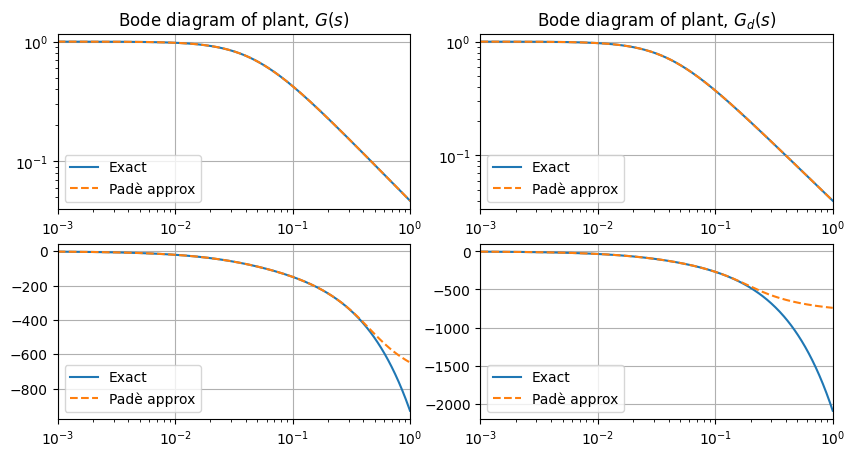
Plant model from mathworks. https://www.mathworks.com/help/control/ug/temperature-control-in-a-heat-exchanger.html. First order + time delay. This example assumes measurable disturbance \(d(t)\), so that they can feed a feedforward controller. This assumption is not made here. The plant is described by the following transfer functions between the output \(Y(s) = T(s)\) (the measurement of temperature) and the control input \(U(s) = V(s)\) (the voltage input to the heat exchanger) and the exogenous input \(D\),

\[y(s) = \underbrace{ \frac{e^{-\tau s}}{a s + 1} u(s)}_{\text{control input}} + \underbrace{\frac{e^{-\tau_d s}}{a_d s + 1} d(s)}_{\text{exogenous input}} = G(s) u(s) + G_d(s) d(s) \ .\]

State-space realization, with \(y(s) = x_1(s) + x_2(s)\), with \(x_1\) from control input, and \(x_2\) from disturbances,

\[\begin{split}\left\{\begin{aligned} \begin{bmatrix} \dot{x}_1 \\ \dot{x}_2 \end{bmatrix} & = \begin{bmatrix} -\frac{1}{a} & \cdot \\ \cdot & -\frac{1}{a_d} \end{bmatrix} \begin{bmatrix} x_1 \\ x_2 \end{bmatrix} + \begin{bmatrix} \frac{1}{a} \\ \cdot \end{bmatrix} u(t-\tau) + \begin{bmatrix} \cdot \\ \frac{1}{a_d} \end{bmatrix} d(t-\tau_d) \\ y & = \begin{bmatrix} \ 1 & 1 \ \end{bmatrix} \begin{bmatrix} x_1 \\ x_2 \end{bmatrix} \end{aligned}\right.\end{split}\]

../../_images/82faac525b07a863d6767ed856fdfeeb80a4e355e51b43f9e0770e43a227f017.png

48.2.3. Control design#

Here a low-order regulator with TF \(R(s)\) is designed for tracking a desired step-input.

The regulator takes the tracking error \(e(t)\) as an input and returns the plant control input \(u(t)\) as its output. Using TF algebra in Laplace domain (for the forced response)

\[\begin{split}\begin{aligned} y & = G u + G_d d = G R e + G_d d = G R ( y_{\text{ref}} - y ) + G_d d \\ e & = y_{\text{ref}} - y = y_{\text{ref}} - G R e - G_d d \\ \end{aligned}\end{split}\]

so that the closed-loop TFs are

\[\begin{split}\begin{aligned} y & = \frac{G R}{1 + G R} y_{\text{ref}} + \frac{G_d}{1 + G R} d =: T(s) y_{\text{ref}} + \frac{G_d}{1 + G R} d \\ e & = \frac{1}{1 + G R} y_{\text{ref}} - \frac{G_d}{1 + G R} d =: S(s) y_{\text{ref}} - \frac{G_d}{1 + G R} d \ . \end{aligned}\end{split}\]

The control input can be written as a function of \(y_{\text{ref}}\) and \(d\) as well

\[u = R e = R y_{\text{ref}} - R y = R y_{\text{ref}} - R G u - R G_d d \ ,\]

so that

\[u = \frac{R}{1 + R G} y_{\text{ref}} - \frac{RG_d}{1 + RG} d \ .\]

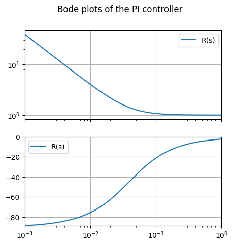
48.2.3.1. PI controller#

With \(e(t) := y_{\text{ref}}(t) - y(t)\)

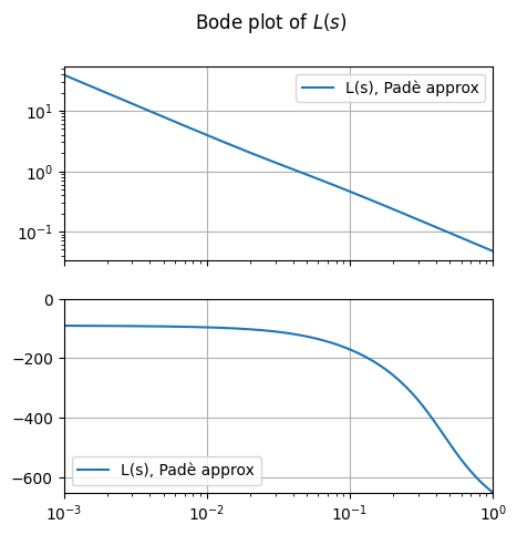
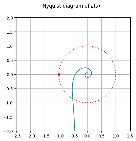
\[\begin{split}\begin{aligned} u(t) & = K_p e(t) + K_i \int_{\tau = 0}^{t} e(\tau) d \tau \\ u(s) & = \left[ K_p + \frac{K_i}{s} \right] e(s) = R(s) e(s) \end{aligned}\end{split}\]

Open-loop TF from error to output \(y(s) = L(s) e(s) = R(s) G(s) e(s)\) reads

\[L(s) = \frac{s K_p + K_i}{s} \frac{e^{-\tau s}}{a s + 1}\]

../../_images/8dbf7fe50c28fe153796d3c5f58119a38bfe2b646a90288c60c4b2126d5e138c.png

Ignoring fixed x limits to fulfill fixed data aspect with adjustable data limits.

../../_images/575abc206ee0ad5b76439d83f5080bece7e6cdb9b7775ed9d775777af2525d14.png

../../_images/01731dd705df285eb478bd817bff4c8ca4de29367818625ab9d89b2987e119ec.png

48.2.3.2. Optimal controller#

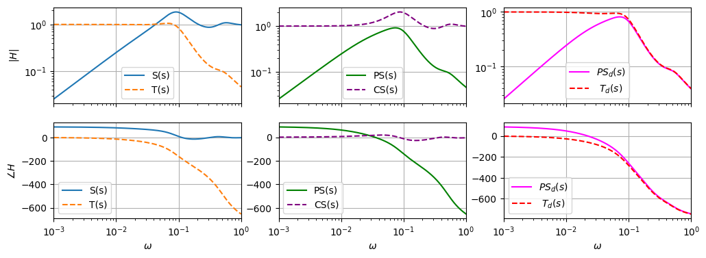
48.2.4. Closed-loop transfer functions - gang of the four#

Show code cell source Hide code cell source

#> Frequency response of the open-loop TF
L_pade_jom = L_pade.frequency_response(omega)

fig, ax = plt.subplots(2,3, figsize=(12,4))
ax[0,0].plot(omega, np.abs( S_jom_complex),       label='S(s)')
ax[0,0].plot(omega, np.abs( T_jom_complex), '--', label='T(s)')
ax[0,0].legend()
ax[0,0].set_xscale('log')
ax[0,0].set_yscale('log')
ax[0,0].set_xlim(omega[0], omega[-1])
ax[0,0].set_xticklabels([])
ax[0,0].grid()

ax[1,0].plot(omega, np.rad2deg(np.unwrap(np.angle( S_jom_complex))),       label='S(s)')
ax[1,0].plot(omega, np.rad2deg(np.unwrap(np.angle( T_jom_complex))), '--', label='T(s)')
ax[1,0].legend()
ax[1,0].set_xscale('log')
ax[1,0].set_xlim(omega[0], omega[-1])
ax[1,0].grid()


ax[0,1].plot(omega, np.abs(PS_jom_complex),       label='PS(s)', color='green')
ax[0,1].plot(omega, np.abs(CS_jom_complex), '--', label='CS(s)', color='purple')
ax[0,1].legend()
ax[0,1].set_xscale('log')
ax[0,1].set_yscale('log')
ax[0,1].set_xlim(omega[0], omega[-1])
ax[0,1].set_xticklabels([])
ax[0,1].grid()

ax[1,1].plot(omega, np.rad2deg(np.unwrap(np.angle(PS_jom_complex))),       label='PS(s)', color='green')
ax[1,1].plot(omega, np.rad2deg(np.unwrap(np.angle(CS_jom_complex))), '--', label='CS(s)', color='purple')
ax[1,1].legend()
ax[1,1].set_xscale('log')
ax[1,1].set_xlim(omega[0], omega[-1])
ax[1,1].grid()


ax[0,2].plot(omega, np.abs(PS_d_jom_complex),       label='$PS_d(s)$', color='magenta')
ax[0,2].plot(omega, np.abs( T_d_jom_complex), '--', label=' $T_d(s)$', color='red')
ax[0,2].legend()
ax[0,2].set_xscale('log')
ax[0,2].set_yscale('log')
ax[0,2].set_xlim(omega[0], omega[-1])
ax[0,2].set_xticklabels([])
ax[0,2].grid()

ax[1,2].plot(omega, np.rad2deg(np.unwrap(np.angle(PS_d_jom_complex))),       label=r'$PS_d(s)$', color='magenta')
ax[1,2].plot(omega, np.rad2deg(np.unwrap(np.angle( T_d_jom_complex))), '--', label=r' $T_d(s)$', color='red')
ax[1,2].legend()
ax[1,2].set_xscale('log')
ax[1,2].set_xlim(omega[0], omega[-1])
ax[1,2].grid()


ax[0,0].set_ylabel(r"$|H|$")
ax[1,0].set_ylabel(r"$\angle H$")
ax[1,0].set_xlabel(r"$\omega$")
ax[1,1].set_xlabel(r"$\omega$")
ax[1,2].set_xlabel(r"$\omega$")


# ax[1].plot(L_pade_jom.omega, np.rad2deg(np.unwrap(L_pade_jom.phase)), label='L(s), Padè approx')
# ax[1].legend()
# ax[1].set_xscale('log')
# ax[1].set_xlim(omega[0], omega[-1])
# ax[1].set_ylim(np.min(np.rad2deg(np.unwrap(L_pade_jom.phase))), np.max([0, np.max(np.rad2deg(np.unwrap(L_pade_jom.phase)))]))
# ax[1].grid()

Text(0.5, 0, '$\\omega$')

../../_images/25ff965da5fae9681e4740632f94b86497d90d7603b8b41f1f5fbc30ea9a6051.png

48.2.4.1. Time-domain response#

0.03996803834887157

../../_images/aa4877005dbde0813490d08ee042868edc38dee19540c0c1587a83b0621382b2.png

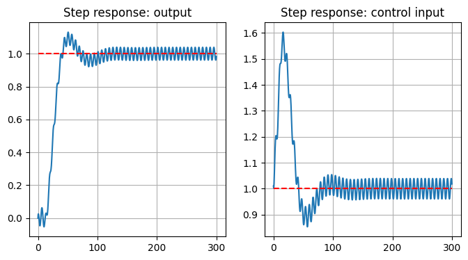
Model error using Padé approximation in time simulation. Only Padé approximation for time delay is supported for state-space representation and time response simulation. Here, the response to a step of closed-loop system with Padé approximation of the time delay is non-zero in \(t \in [0, \tau]\), but shows “small-amplitude” oscillations.

Effect of the disturbances. Here the harmonic disturbances have frequency \(\omega_d\) much larger than the cutting frequency \(\omega_c\). Thus, \(d\) produces the output \(y_d(\omega_d) = T_d(\omega_d) d(\omega_d)\), with gain \(|G(\omega_d)| \simeq .04\) Thus, even with a disturbance \(d\) with the same amplitude as the reference step signal, the oscillations around the desired output have “small” amplitude, \(y_d \simeq A_d \cos( \omega_d t + \varphi_d)\), with \(A_d = |T_d(\omega_d)| |d(\omega_d)| \simeq .04 |d(\omega_d)|\).