44. Closed-loop control: requirements and performance#

Requirement/Performance

Stability

Nyquist criterion on the open-loop TF \(L(s)\)

Robustness

Stability margins

Reference tracking

Type of the system. Integrators in open-loop TF \(L(s)\)

Measurement noise suppression

Input load

Input noise suppression

Transient performance

Let the transfer function of the system be

\[\mathbf{y} = \mathbf{G} \mathbf{u} + \mathbf{G}_d \mathbf{d} + \mathbf{G}_n \mathbf{n} \ ,\]

linking the control input \(\mathbf{u}\), and the exogenous inputs ( process disturbances \(\mathbf{d}\), and measurement noise \(\mathbf{n}\)) to the output \(\mathbf{y}\). Let control disturbance \(\Delta \mathbf{u}\) on the ideal control \(\mathbf{u}_c\) be additive, \(\mathbf{u} = \mathbf{u}_c + \Delta \mathbf{u}\). Let \(\mathbf{F}\) be a feed-forward system from reference \(\mathbf{r}\) to the reference output \(\mathbf{y}_{\text{ref}}\) that is compared with the output of the system \(\mathbf{y}\) to define the error \(\mathbf{e} = \mathbf{y}_{\text{ref}} - \mathbf{y}\) feeding the regulator \(\mathbf{R}\).

Transfer function of the closed-loop system

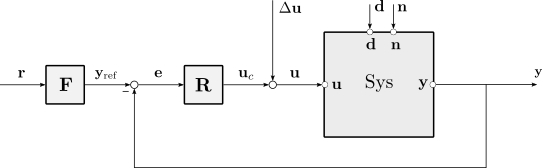
Fig. 44.1 Block diagram of the closed-loop system#

Closed-loop performance usually deals with the relation between the output \(\mathbf{y}\), the tracking error \(\mathbf{e}\), and the ideal control input \(\mathbf{u}_c\) (the output of he regulator; that’s what we need to care about for controller response, performance, saturation,…) w.r.t. the reference signal \(\mathbf{r}\) and the exogenous inputs \(\Delta \mathbf{u}\), \(\mathbf{d}\), \(\mathbf{r}\), in terms of:

  • tracking of the reference

  • control performance

  • disturbance suppression/noise rejection (on both the output and the input control)

For a MIMO

\[\begin{split} \begin{bmatrix} \mathbf{y} \\ \mathbf{e} \\ \mathbf{u}_c \end{bmatrix} = \begin{bmatrix} \left[ \mathbf{I} + \mathbf{G} \mathbf{R} \right]^{-1} & \cdot & \cdot \\ \cdot & \left[ \mathbf{I} + \mathbf{G} \mathbf{R} \right]^{-1} & \cdot \\ \cdot & \cdot &\left[ \mathbf{I} + \mathbf{R} \mathbf{G} \right]^{-1} \end{bmatrix} \begin{bmatrix} \mathbf{G} \mathbf{R} \mathbf{F} & \mathbf{G} & \mathbf{G}_d & \mathbf{G}_n \\ \mathbf{F} & - \mathbf{G} & - \mathbf{G}_d & - \mathbf{G}_n \\ \mathbf{R} \mathbf{F} & - \mathbf{R} \mathbf{G} & - \mathbf{R} \mathbf{G}_d & - \mathbf{R} \mathbf{G}_n \\ \end{bmatrix} \begin{bmatrix} \mathbf{r} \\ \Delta \mathbf{u} \\ \mathbf{d} \\ \mathbf{n} \end{bmatrix} \ . \end{split}\]

For a SISO

\[\begin{split} \begin{bmatrix} y \\ e \\ u_c \end{bmatrix} = \frac{1}{1+GR} \begin{bmatrix} GRF & G & G_d & G_n \\ F & - G & - G_d & - G_n \\ R F & - R G & - R G_d & - R G_n \end{bmatrix} \begin{bmatrix} r \\ \Delta u \\ d \\ n \end{bmatrix} \ . \end{split}\]

Two-degrees of freedom problem. Typical design procedure:

  • Design \(R\) to provide load/noise performance

  • Design \(F\) to provide tracking performance

Simplified model. If

  • there’s no feed-forward, i.e. \(\mathbf{F} = \mathbf{I}\) or \(F = 1\) for a SISO,

  • the measurement noise is additive on an ideal output, the TF is \(\mathbf{y} = \mathbf{G} \mathbf{u} + \mathbf{G}_d \mathbf{d} + \mathbf{n}\), i.e.\(\mathbf{G}_n = \mathbf{I}\) or \(G_n(s) = 1\) for a SISO,

for a MIMO

\[\begin{split} \begin{bmatrix} \mathbf{y} \\ \mathbf{e} \\ \mathbf{u}_c \end{bmatrix} = \begin{bmatrix} \left[ \mathbf{I} + \mathbf{G} \mathbf{R} \right]^{-1} & \cdot & \cdot \\ \cdot & \left[ \mathbf{I} + \mathbf{G} \mathbf{R} \right]^{-1} & \cdot \\ \cdot & \cdot & \left[ \mathbf{I} + \mathbf{R} \mathbf{G} \right]^{-1} \end{bmatrix} \begin{bmatrix} \mathbf{G} \mathbf{R} & \mathbf{G} & \mathbf{G}_d & \mathbf{I} \\ \mathbf{I} & - \mathbf{G} & - \mathbf{G}_d & - \mathbf{I} \\ \mathbf{R} & - \mathbf{R} \mathbf{G} & - \mathbf{R} \mathbf{G}_d & - \mathbf{R} \\ \end{bmatrix} \begin{bmatrix} \mathbf{r} \\ \Delta \mathbf{u} \\ \mathbf{d} \\ \mathbf{n} \end{bmatrix} \ , \end{split}\]

and for a SISO

\[\begin{split} \begin{bmatrix} y \\ e \\ u_c \end{bmatrix} = \frac{1}{1+GR} \begin{bmatrix} G R & G & G_d & 1 \\ 1 & - G & - G_d & - 1 \\ R & - R G & - R G_d & - R \end{bmatrix} \begin{bmatrix} r \\ \Delta u \\ d \\ n \end{bmatrix} \ . \end{split}\]

For a SISO, beside process noise \(\mathbf{d}\) that may have its own dynamics, the performance of the closed loop system is defined by 4 transfer functions only, “the gang of the 4”,

  • sensitivity function (\(\mathbf{y}(\mathbf{n})\), \(\mathbf{e}(\mathbf{r})\), \(\mathbf{e}(\mathbf{n})\))

    \[S = \frac{1}{1 + GR} \ ,\]
  • complementary sensitivity (\(\mathbf{y}(\mathbf{r})\), \(\mathbf{u}_c(\Delta \mathbf{u})\))

    \[T = \frac{GR}{1 + GR} \ ,\]
  • load sensitivity (\(\mathbf{y}(\Delta \mathbf{u})\), \(\mathbf{e}(\Delta \mathbf{u})\))

    \[PS = \frac{G}{1 + GR} \ ,\]
  • noise sensitivity (\(\mathbf{u}_c(\mathbf{r})\), \(\mathbf{u}_c(\mathbf{n})\))

    \[CS = \frac{R}{1 + GR} \ ,\]
Details

Output.

\[\begin{split}\begin{aligned} \mathbf{y} & = \mathbf{G} \mathbf{u} + \mathbf{G}_d \mathbf{d} + \mathbf{G}_n \mathbf{n} = \\ & = \mathbf{G} \left( \mathbf{u}_c + \Delta \mathbf{u} \right) + \mathbf{G}_d \mathbf{d} + \mathbf{G}_n \mathbf{n} = \\ & = \mathbf{G} \mathbf{R} \mathbf{e} + \mathbf{G} \Delta \mathbf{u} + \mathbf{G}_d \mathbf{d} + \mathbf{G}_n \mathbf{n} = \\ & = \mathbf{G} \mathbf{R} \left( \mathbf{y}_{\text{ref}} - \mathbf{y} \right) + \mathbf{G} \Delta \mathbf{u} + \mathbf{G}_d \mathbf{d} + \mathbf{G}_n \mathbf{n} = \\ & = \mathbf{G} \mathbf{R} \mathbf{F} \mathbf{r} - \mathbf{G} \mathbf{R} \mathbf{y} + \mathbf{G} \Delta \mathbf{u} + \mathbf{G}_d \mathbf{d} + \mathbf{G}_n \mathbf{n} \ , \end{aligned}\end{split}\]

and thus

\[\begin{split}\begin{aligned} \mathbf{y} & = \left[ \mathbf{I} + \mathbf{G}\mathbf{R} \right]^{-1} \mathbf{G} \mathbf{R} \mathbf{F} \, \mathbf{r} + \\ & + \left[ \mathbf{I} + \mathbf{G}\mathbf{R} \right]^{-1} \mathbf{G} \, \Delta \mathbf{u} + \\ & + \left[ \mathbf{I} + \mathbf{G}\mathbf{R} \right]^{-1} \mathbf{G}_d \, \mathbf{d} + \\ & + \left[ \mathbf{I} + \mathbf{G}\mathbf{R} \right]^{-1} \mathbf{G}_n \, \mathbf{n} \ . \end{aligned}\end{split}\]

Error.

\[\begin{split}\begin{aligned} \mathbf{e} & = \mathbf{F} \mathbf{r} - \mathbf{y} = \\ & = \mathbf{F} \mathbf{r} - \left( \mathbf{G} \mathbf{u} + \mathbf{G}_d \mathbf{d} + \mathbf{G}_n \mathbf{n} \right) = \\ & = \mathbf{F} \mathbf{r} - \mathbf{G} \mathbf{u}_c - \mathbf{G} \Delta \mathbf{u} - \mathbf{G}_d \mathbf{d} - \mathbf{G}_n \mathbf{n} = \\ & = \mathbf{F} \mathbf{r} - \mathbf{G} \mathbf{R} \mathbf{e} - \mathbf{G} \Delta \mathbf{u} - \mathbf{G}_d \mathbf{d} - \mathbf{G}_n \mathbf{n} \ , \end{aligned}\end{split}\]

and thus

\[\begin{split}\begin{aligned} \mathbf{e} & = \left[ \mathbf{I} + \mathbf{G} \mathbf{R} \right]^{-1} \mathbf{F} \, \mathbf{r} + \\ & - \left[ \mathbf{I} + \mathbf{G} \mathbf{R} \right]^{-1} \mathbf{G} \, \Delta \mathbf{u} + \\ & - \left[ \mathbf{I} + \mathbf{G} \mathbf{R} \right]^{-1} \mathbf{G}_d \, \mathbf{d} + \\ & - \left[ \mathbf{I} + \mathbf{G} \mathbf{R} \right]^{-1} \mathbf{G}_r \, \mathbf{r} \ . \end{aligned}\end{split}\]

Input.

\[\begin{split}\begin{aligned} \mathbf{u}_c & = \mathbf{R} \mathbf{F} \mathbf{r} - \mathbf{R} \mathbf{y} = \\ & = \mathbf{R} \mathbf{F} \mathbf{r} - \mathbf{R} \left( \mathbf{G} \mathbf{u} + \mathbf{G}_d \mathbf{d} + \mathbf{G}_n \mathbf{n} \right) = \\ & = \mathbf{R} \mathbf{F} \mathbf{r} - \mathbf{R} \mathbf{G} \mathbf{u}_c - \mathbf{R} \mathbf{G} \Delta \mathbf{u} - \mathbf{R} \left( \mathbf{G}_d \mathbf{d} + \mathbf{G}_n \mathbf{n} \right) \ , \end{aligned}\end{split}\]

and thus

\[\begin{split}\begin{aligned} \mathbf{u}_c & = \left[ \mathbf{I} + \mathbf{R} \mathbf{G} \right]^{-1} \mathbf{R} \mathbf{F} \, \mathbf{r} + \\ & - \left[ \mathbf{I} + \mathbf{R} \mathbf{G} \right]^{-1} \mathbf{R} \mathbf{G} \, \Delta \mathbf{u} + \\ & - \left[ \mathbf{I} + \mathbf{R} \mathbf{G} \right]^{-1} \mathbf{R} \mathbf{G}_d \, \mathbf{d} + \\ & - \left[ \mathbf{I} + \mathbf{R} \mathbf{G} \right]^{-1} \mathbf{R} \mathbf{G}_r \, \mathbf{r} \ . \end{aligned}\end{split}\]

Algebraic constraint on sensitivity and complementary sensitivity. It’s not possible to make \(S(s)\) and \(T(s)\) small at the same time, as

\[S(s) + T(s) = 1\]

Usually,

  • \(|S(j \omega)|\) small at low frequency \(\omega\) to get small error in the band of the reference and filtering low-frequency measurement noise on the inp

  • \(|T(j \omega)|\) small at high frequency \(\omega\) to filter high-frequency noise from \(\Delta u\) to \(u\) (usually reference signal \(r\) has no high-frequency content, so there should be little issues in filtering out the effect of reference signal to the output).