Inverted pendulum

48.3. Inverted pendulum#

48.3.1. Equations of motion with Lagrangian mechanics#

48.3.1.1. Non-linear equations#

Second-order dynamical equation of the mechanical system reads

\[m \ell^2 \ddot{\theta} + c \dot{\theta} = m g \ell \sin \theta + C \ .\]

Equilibrium conditions of unforced system (\(C = 0\)) are found for \(\overline{\theta}_1 = 0\), \(\overline{\theta}_2 = \pi\). The first equilibrium is unstable, the second equilibrium is stable. Around the second equilibrium, the linearized equation becomes

\[m \ell^2 \ddot{\theta} + c \dot{\theta} + m g \ell \theta = C \ ,\]

so that, for under-damped systems, it’s possible to define the natural frequency of the undamped system \(\omega_n^2 = \frac{g}{\ell}\), and the damping coefficient \(\xi\)

as, by definition

\[2 \xi \omega_n := \frac{c}{m\ell^2} \]

\[\xi = \frac{c}{2 m \ell^2 \omega_n} = \frac{c}{2 m \ell^2 \sqrt{\frac{g}{\ell}}}\]

48.3.1.2. Equilibria#

48.3.1.3. Linearized equations around equilibria#

Linearized equation around the stable equilibrium. First-order system equation around the stable equilibium becomes

\[\begin{split}\begin{bmatrix} \dot{\theta} \\ \dot{\Omega} \end{bmatrix} = \begin{bmatrix} 0 & 1 \\ - \omega_n^2 & - 2 \omega_n \xi \end{bmatrix} \begin{bmatrix} \theta \\ \Omega \end{bmatrix} + \begin{bmatrix} 0 \\ \frac{1}{m \ell^2} \end{bmatrix} C \ .\end{split}\]

Linearized equation around the unstable equilibrium. First-order system equation around the unstable equilibium becomes

\[\begin{split}\begin{aligned} \begin{bmatrix} \dot{\theta} \\ \dot{\Omega} \end{bmatrix} & = \begin{bmatrix} 0 & 1 \\ \omega_n^2 & - 2 \omega_n \xi \end{bmatrix} \begin{bmatrix} \theta \\ \Omega \end{bmatrix} + \begin{bmatrix} 0 \\ \frac{1}{m \ell^2} \end{bmatrix} C \\ y & = \begin{bmatrix} \ 1 & 0 \ \end{bmatrix} \begin{bmatrix} \theta \\ \Omega \end{bmatrix} \ . \end{aligned}\end{split}\]

This the equation we’re interested in, when studying the inverted pendulum system.

48.3.1.4. Augmented sytem for tracking reference signal#

Let \(\mathbf{y}_{\text{ref}}\) a reference signal. An augmented system can be defined in order to used optimal control. Let

\[\begin{split}\begin{aligned} \dot{\mathbf{x}} & = \mathbf{A} \mathbf{x} + \mathbf{B} \mathbf{u} \\ \mathbf{y} & = \mathbf{C} \mathbf{x} + \mathbf{D} \mathbf{u} \end{aligned}\end{split}\]

the state-space representation of the plant. Let \(\mathbf{y}_{\text{ref}}\) a desired output and the integral error

\[\mathbf{e}_{\text{int}}(t) := \int_{\tau=0}^{t} \left\{ \mathbf{y}(\tau) - \mathbf{y}_{\text{ref}}(\tau) \right\} d \tau \ ,\]

as a new state with dynamical equation

\[\dot{\mathbf{e}}_{\text{int}} = \mathbf{y}(t) - \mathbf{y}_{\text{ref}}(t) = \mathbf{C} \mathbf{x} + \mathbf{D} \mathbf{u} - \mathbf{y}_{\text{ref}} \ .\]

The optimal control is applied to the augmented system

\[\begin{split}\underbrace{\begin{bmatrix} \dot{\mathbf{x}} \\ \dot{\mathbf{e}}_{\text{int}} \end{bmatrix}}_{\dot{\mathbf{z}}} = \underbrace{\begin{bmatrix} \mathbf{A} & \cdot \\ \mathbf{C} & \cdot \end{bmatrix}}_{\hat{\mathbf{A}}} \underbrace{\begin{bmatrix} \mathbf{x} \\ \mathbf{e}_{\text{int}} \end{bmatrix}}_{\mathbf{z}} + \underbrace{\begin{bmatrix} \mathbf{B} \\ \mathbf{D} \end{bmatrix}}_{\hat{\mathbf{B}}_u} \mathbf{u} + \underbrace{\begin{bmatrix} \cdot \\ -\mathbf{I} \end{bmatrix}}_{\hat{\mathbf{B}}_{ref}} \mathbf{y}_{ref}\end{split}\]

\[\mathbf{y} = \hat{\mathbf{C}} \mathbf{z} + \hat{\mathbf{D}}_u \mathbf{u} \ .\]

Optimal control framework provides the opitmal gain matrix \(\hat{\mathbf{K}}\), so that \(\mathbf{u} = - \hat{\mathbf{K}} \mathbf{z}\) and the closed loop system becomes

\[\begin{split}\begin{aligned} \dot{\mathbf{z}} & = \left( \hat{\mathbf{A}} - \hat{\mathbf{B}}_u \hat{\mathbf{K}} \right) \mathbf{z} + \hat{\mathbf{B}}_{ref} \mathbf{y}_{ref} \\ \mathbf{y} & = \left( \hat{\mathbf{C}} - \hat{\mathbf{D}}_u \mathbf{K} \right) \mathbf{z} \ . \end{aligned}\end{split}\]

If the output of the system is the angle \(\theta(t)\), with reference signal \(\mathbf{y}_{\text{ref}} = \theta_{\text{ref}}\), the dynamical system is a SISO system, whose state-space representation is

…

48.3.2. Libraries#

0.10.2

48.3.3. Plant dynamical equations#

[ 0.        +0.j -7.07395639+0.j  6.93388498+0.j]

48.3.4. Control#

48.3.4.1. Optimal control for full-state feedback#

State-space representation of the open-loop system from the tracking error \(\mathbf{e}\) to the output \(\mathbf{y}\) reads

\[\begin{split}\left\{\begin{aligned} \dot{\mathbf{x}} & = \left( \mathbf{A} - \mathbf{B} \mathbf{K}_{\mathbf{x}} \right) \mathbf{x} - \mathbf{B} \mathbf{K}_{\mathbf{e}} \mathbf{e}_{\text{int}} \\ \dot{\mathbf{e}}_{\text{int}} & = \mathbf{e} \\ \mathbf{y} & = \left( \mathbf{C} - \mathbf{D} \mathbf{K}_{\mathbf{x}} \right) \mathbf{x} - \mathbf{D} \mathbf{K}_{\mathbf{e}} \mathbf{e}_{\text{int}} \ , \end{aligned}\right.\end{split}\]

or

\[\begin{split}\left\{\begin{aligned} \begin{bmatrix} \dot{\mathbf{x}} \\ \dot{\mathbf{e}}_{\text{int}} \end{bmatrix} & = \begin{bmatrix} \mathbf{A} - \mathbf{B} \mathbf{K}_{\mathbf{x}} & - \mathbf{B} \mathbf{K}_{\mathbf{e}} \\ \cdot & \cdot \end{bmatrix} \begin{bmatrix} \mathbf{x} \\ \mathbf{e}_{\text{int}} \end{bmatrix} + \begin{bmatrix} \cdot \\ \mathbf{I} \end{bmatrix} \mathbf{e} \\ \mathbf{y} & = \begin{bmatrix} \mathbf{C} - \mathbf{D} \mathbf{K}_{\mathbf{x}} & - \mathbf{D} \mathbf{K}_{\mathbf{e}} \end{bmatrix} \begin{bmatrix} \mathbf{x} \\ \mathbf{e}_{\text{int}} \end{bmatrix} \end{aligned}\right.\end{split}\]

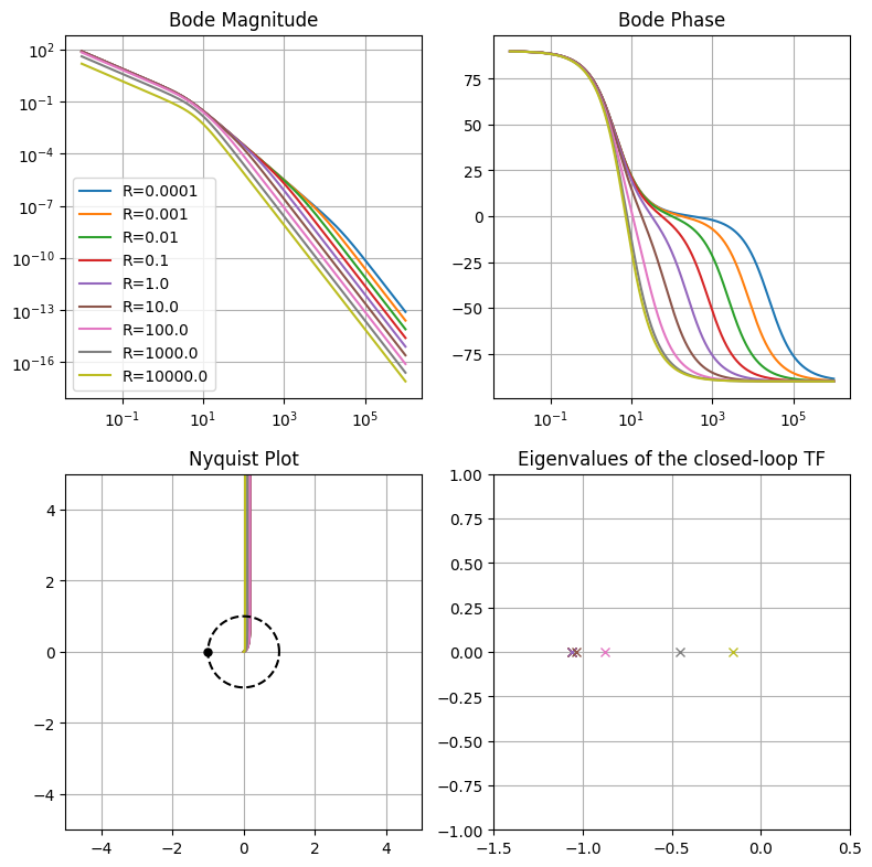
48.3.4.1.1. Sensitivity to control weight#

For a given weight matrix on the augmented state \(\mathbf{Q}\), here the sensitivity to the value of the control weight \(\mathbf{R} = [ \ r \ ]\) is investigated. Here, the output is the angle \(\theta\) of the inverted pendulum w.r.t. the unstable equilibrium.

Bode and Nyquist diagram of the stabilized1 open-loop TF are shown, along with the eigenvalues of the closed loop system, with the reference signal as input.

Show code cell source Hide code cell source

# LQR Weights
Q = np.diag([10, 1, 10]) # Penalize angle error more than angular velocity
# R_values = np.linspace(0.001, .01, 4)  # [0.001, 0.01, 0.1]
R_values = np.logspace(-4, 4, 9)

omega_freq = np.logspace(-2, 6, 500)

fig, ax = plt.subplots(2,2, figsize=(8, 8))

for R in R_values:

    # Compute LQR Gain
    # K, S, E = ct.lqr(A, B, Q, R)
    Ka, Sa, Ea = ct.lqr(sys_aug, Q, R)

    #> Loop transfer function L(s) = K * (sI - A)^-1 * B
    #> Open-loop TF, L(s) = G(s) R(s), with R(s) = K
    # from the error to the output
    A_ol = np.block([
        [     A - B @ Ka[:,:2], - B @ Ka[:,2:]],
        [      np.zeros((1,2)), np.zeros((1, 1))]
    ])
    B_ol = np.block([[.0], [.0], [1.]])
    C_ol = np.block([[ C - D @ Ka[:,:2], - D @ Ka[:,2]]])
    D_ol = np.zeros((1,1))
    sys_ol = ct.ss(A_ol, B_ol, C_ol, D_ol)

    #> Closed-loop TF
    # from the disturbance signal to the output
    # Simulate closed-loop response with reference input
    A_cl = Aa - Ba @ Ka
    B_ref = np.array([[0], [0], [-1]])
    C_cl = np.array([[1, 0, 0]])
    D_cl = np.zeros((1, 1))

    sys_cl = ct.ss(A_cl, B_ref, C_cl, D_cl)

    evals_cl = ct.poles(sys_cl)

    #> Frequency response
    mag_L, phase_L, omega_L = ct.frequency_response(sys_ol, omega_freq)

    #> Plots
    #> Bode plots (first line) of L(s)
    ax[0,0].loglog(omega_L, mag_L, label=f'R={R}')
    ax[0,1].semilogx(omega_L, np.degrees(phase_L), label=f'R={R}')
    #> Nyquist diagram of L(s)
    ax[1,0].plot(mag_L*np.cos(phase_L), mag_L*np.sin(phase_L), label=f'R={R}')
    #> Eigenvalues of the closed-loop system
    ax[1,1].plot(np.real(evals_cl), np.imag(evals_cl), 'x', label=f'R={R}')

#> Critical point and circle in Nyquist plot
theta_v = np.linspace(0, 2*np.pi, 100)
ax[1,0].plot([-1], [0], 'o', ms=5, color="black")
ax[1,0].plot(np.cos(theta_v), np.sin(theta_v), '--', color="black")

#> Formatting plots
ax[0,0].set_title('Bode Magnitude'); ax[0,0].grid(True); ax[0,0].legend()
ax[0,1].set_title('Bode Phase'); ax[0,1].grid(True)
ax[1,0].set_title('Nyquist Plot'); ax[1,0].grid(True); ax[1,0].set_aspect('equal'); ax[1,0].set_xlim([-5, 5]); ax[1,0].set_ylim([-5, 5])
ax[1,1].set_title('Eigenvalues of the closed-loop TF'); ax[1,1].grid(True); ax[1,1].set_aspect('equal')
ax[1,1].set_xlim([-1.5, .5]); ax[1,1].set_ylim([-1., 1.])

fig.set_tight_layout(True)

plt.show()

../../_images/2e0dca1466f04300cfb21662dbb2b95ea7dc8568fc6341abe81310f6746104d9.png

48.3.4.2. Optimal observer#

System equations, without disturbances/noise

\[\begin{split}\left\{\begin{aligned} \dot{\mathbf{x}} & = \mathbf{A} \mathbf{x} + \mathbf{B} \mathbf{u} \\ \mathbf{y} & = \mathbf{C} \mathbf{x} + \mathbf{D} \mathbf{u} \ , \end{aligned}\right.\end{split}\]

Observer (state estimator) equations

\[\begin{split}\left\{\begin{aligned} \hat{\mathbf{y}} & = \mathbf{C} \hat{\mathbf{x}} + \mathbf{D} \mathbf{u} \\ \dot{\hat{\mathbf{x}}} & = \mathbf{A} \hat{\mathbf{x}} + \mathbf{B} \mathbf{u} + \mathbf{L} \left( \mathbf{y} - \hat{\mathbf{y}} \right) \\ & = \left( \mathbf{A} - \mathbf{L} \mathbf{C} \right) \hat{\mathbf{x}} + \mathbf{L} \mathbf{C} \mathbf{x} + \mathbf{B} \mathbf{u} \ , \end{aligned}\right.\end{split}\]

so that the dynamical equation of the error \(\boldsymbol\varepsilon := \hat{\mathbf{x}} - \mathbf{x}\) reads

\[\dot{\boldsymbol\varepsilon} = \left( \mathbf{A} - \mathbf{L} \mathbf{C} \right) \boldsymbol\varepsilon \ .\]

The dynamical equations of the augmented system, plant+observer, reads

\[\begin{split}\begin{bmatrix} \dot{\mathbf{x}} \\ \dot{\boldsymbol\varepsilon} \end{bmatrix} = \begin{bmatrix} \mathbf{A} & \mathbf{0} \\ \mathbf{0} & \mathbf{A} - \mathbf{L} \mathbf{C} \end{bmatrix} \begin{bmatrix} \mathbf{x} \\ \boldsymbol\varepsilon \end{bmatrix} + \begin{bmatrix} \mathbf{B} \\ \mathbf{0} \end{bmatrix} \mathbf{u} \ ,\end{split}\]

and the observer design here is the design of a matrix \(\mathbf{L}\) that makes the dynamics of the error \(\boldsymbol\varepsilon\), and thus the matrix \(\mathbf{A} - \mathbf{L} \mathbf{C}\), asymptotically stable.

48.3.4.2.1. State estimator with process and measurement noise#

\[\begin{split}\left\{\begin{aligned} \dot{\mathbf{x}} & = \mathbf{A} \mathbf{x} + \mathbf{B} \mathbf{u} + \mathbf{B}_d \mathbf{d}\\ \mathbf{y} & = \mathbf{C} \mathbf{x} + \mathbf{D} \mathbf{u} + \mathbf{D}_d \mathbf{d} + \mathbf{D}_r \mathbf{r} \ , \end{aligned}\right.\end{split}\]

The state estimator problem with \(\mathbf{D}_d = \mathbf{0}\) and \(\mathbf{D}_\mathbf{r} = \mathbf{I}\) can be solved with the function \(\texttt{lqe}\) of the \(\texttt{control}\) library,

\[\begin{split}\begin{aligned} & \texttt{control.lqe(sys, Edd, Err, Edr)} \\ & \texttt{control.lqe(A, Bd, C, Edd, Err, Edr)} \\ \end{aligned}\end{split}\]

[[13.87503766]
 [96.258335  ]]

"\n#> Method 2.\n# Use LQR duality: lqe(A, B, C, V, W) is dual to lqr(A.T, C.T, V, W)\n# Note: we use C.T because it replaces B in the dual problem\nL_transposed, P, E = ct.lqr(A.T, C.T, V, W)\n\n# The actual observer gain is the transpose of the 'feedback' result\nL = L_transposed.T\n"

48.3.4.3. Combination of controller and observer - separation principle#

48.3.4.4. Properties of control#

…

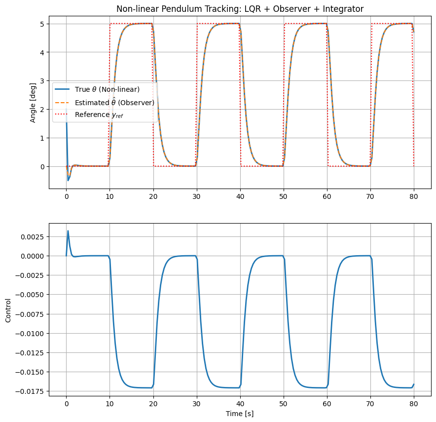
48.3.5. Verifying control on non-linear system#

48.3.5.1. Reference tracking on the non-linear system#

Here the control system is tested on the non-linear system for tracking a reference square wave signal.

Non-linear equations of the plant

\[\begin{split}\begin{aligned} \dot{\mathbf{x}} & = \mathbf{f}(\mathbf{x}, \mathbf{u}) \\ \mathbf{y} & = \mathbf{C} \mathbf{x} + \mathbf{D} \mathbf{u} \end{aligned}\end{split}\]

Observer

\[\dot{\boldsymbol\varepsilon} = \left( \mathbf{A} - \mathbf{L} \mathbf{C} \right) \boldsymbol\varepsilon\]

Integral error

\[\dot{\mathbf{e}}_{\text{int}} = \mathbf{y} - \mathbf{y}_{\text{ref}}\]

Proportional control

\[\mathbf{u} = - \mathbf{K}_{\mathbf{x}} \mathbf{x} - \mathbf{K}_{\mathbf{x}} \boldsymbol\varepsilon - \mathbf{K}_{\mathbf{e}} \mathbf{e}_{\text{int}} \ .\]

../../_images/1764bb50a395029c4192eba83e9471af5919e54052c95c11768aaf32f1133191.png

1: After the optimal control gain matrix \(\mathbf{K}\) has been computed, i.e. it’s not surprising that this open-loop system is stable.