18.2.4.4. \(t\)-test#
Un \(t\)-test è un test di verifica delle ipotesi nel quale la statistica test ha una distribuzione \(\mathbf{t}\) di Student sotto l’ipotesi nulla \(\text{H}_0\),
18.2.4.4.1. \(t\)-test per un campione#
Il \(t\)-test per un campione è un test di verifica del valore di un parametro, per la media di una variabile casuale sotto un’opportuna ipotesi nulla \(\text{H}_0\). Il parametro \(t\),
confronta la distanza della media \(\bar{x}\) del campione dal valore medio \(\mu_0\) della distribuzione \(p(x|\text{H}_0)\), con la deviazione standard del campione \(s\) opportunamente scalata della grandezza del campione \(n\).
Se le osservazioni della variabile casuale sono indipdendenti tra di loro, allora \(t\) è una variabile casuale che tende a una variabile normale \(\mathscr{N}(0,1)\) per il teorema del limite centrale todo link a una sezione sul campionamento
# Example
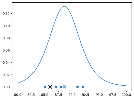
import numpy as np
from scipy.stats import ttest_1samp, t
import matplotlib.pyplot as plt
# Test statistics has expected value mu0 under H0 hypotesis
mu0 = 86. # Expeceted value of the test statistics under H0
sigma = 0.05 # Significance level
# Sample data: test scores from two classes
sample = [88, 92, 85, 91, 87]
n_s = len(sample)
mu_s = np.sum(sample)/n_s
s_s = ( np.sum((sample-mu_s)**2)/(n_s-1) )**.5
print("Sample statistics:")
print(f" sample avg : {mu_s}")
print(f" sample std.dev: {s_s}")
# Perform independent t-test
t_statistic, p_value = ttest_1samp(sample, mu0)
print(f"\n1-sample t-test")
print(f" t-Statistic: {t_statistic}")
print(f" p-Value : {p_value}")
# Interpretation
if p_value < sigma:
print("\n> Reject the null hypothesis, H0: the means of the two classes are significantly different.")
else:
print("\n> Fail to reject the null hypothesis, H0: no significant difference in means between the classes.")
x_plot = np.arange(80, 100, .01)
t_pdf_plot = t.pdf(x_plot, n_s, mu_s, s_s)
plt.figure()
plt.plot(x_plot, t_pdf_plot, color=plt.cm.tab10(0))
plt.plot(sample, np.zeros(n_s), 'o', color=plt.cm.tab10(0))
plt.plot(mu_s, 0., 'x', color=plt.cm.tab10(0), markersize=10, markeredgewidth=2)
plt.plot(mu0 , 0., 'x', color='black' , markersize=10, markeredgewidth=2)
Sample statistics:
 sample avg    : 88.6
 sample std.dev: 2.8809720581775866

1-sample t-test
 t-Statistic: 2.017991366836461
 p-Value    : 0.11375780482862627

> Fail to reject the null hypothesis, H0: no significant difference in means between the classes.
[<matplotlib.lines.Line2D at 0x7fb372a7e910>]
18.2.4.4.2. \(t\)-test per due campioni#
test con varianza uguale (o simile), t-test/test con varianza diversa, Welch
campioni indipendenti/campioni dipendenti (paired samples)
18.2.4.4.2.1. \(t\)-test per due variabili indipendenti, con varianza simile e stesso numero di osservazioni#
Nell’ipotesi che i campioni siano ottenuti da due variabili indipendenti, i risultati ottenuti nella sezione sulla combinazione di variabili casuali
il valore atteso della somma/differenza di variabili casuali indipendenti è uguale alla somma/differenza dei valori attesi delle singole variabili
la varianza della somma/differenza di variabili casuali indipendenti è uguale alla somma delle varianze delle singole variabili.
Il \(t\)-test per due campioni equivale al \(t\)-test per un campione uguale alla differenza delle osservazioni nei due campioni,
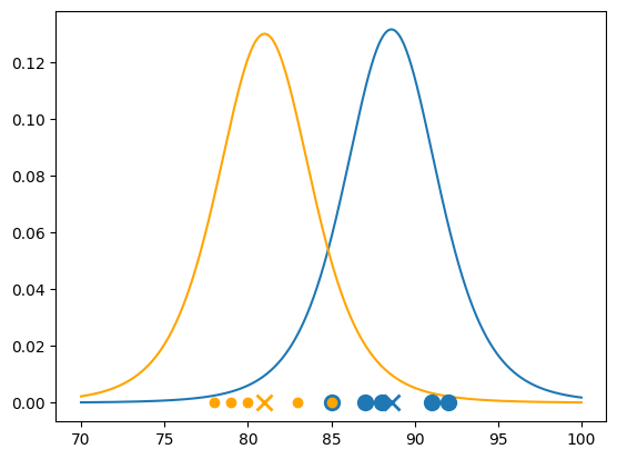
# Example

import numpy as np
from scipy.stats import ttest_ind

# Significance level
sigma = 0.05

# Sample data: test scores from two classes
class_A = [88, 92, 85, 91, 87]
class_B = [78, 85, 80, 83, 79]

nA = len(class_A); mu_A = np.sum(class_A)/nA; sA = ( np.sum((class_A-mu_A)**2)/(nA-1) )**.5
nB = len(class_B); mu_B = np.sum(class_B)/nB; sB = ( np.sum((class_B-mu_B)**2)/(nB-1) )**.5

print("Sample statistics:")
print("Sample A")
print(f" sample avg    : {mu_A}")
print(f" sample std.dev: {sA}")
print("Sample B")
print(f" sample avg    : {mu_B}")
print(f" sample std.dev: {sB}")


# Perform independent t-test
t_statistic, p_value = ttest_ind(class_A, class_B)


print(f"\ns-sample t-test")
print(f" t-Statistic: {t_statistic}")
print(f" p-Value    : {p_value}")

print((mu_A-mu_B)/((sA**2 + sB**2)/nA)**.5)

# Interpretation
if p_value < sigma:
    print("\nReject the null hypothesis: The means of the two classes are significantly different.")
else:
    print("\nFail to reject the null hypothesis: No significant difference in means between the classes.")

x_plot = np.arange(70, 100, .01)
t_pdf_A = t.pdf(x_plot, nA, mu_A, sA)
t_pdf_B = t.pdf(x_plot, nB, mu_B, sB)

plt.figure()
plt.plot(x_plot, t_pdf_A, color=plt.cm.tab10(0))
plt.plot(x_plot, t_pdf_B, color='orange')
plt.plot(class_A, np.zeros(nA), 'o', color=plt.cm.tab10(0), markersize=10)
plt.plot(class_B, np.zeros(nB), 'o', color='orange'       )
plt.plot(mu_A, 0., 'x', color=plt.cm.tab10(0), markersize=10, markeredgewidth=2)
plt.plot(mu_B, 0., 'x', color='orange'       , markersize=10, markeredgewidth=2)
Sample statistics:
Sample A
 sample avg    : 88.6
 sample std.dev: 2.8809720581775866
Sample B
 sample avg    : 81.0
 sample std.dev: 2.9154759474226504

s-sample t-test
 t-Statistic: 4.146139914483853
 p-Value    : 0.0032260379191180397
4.146139914483853

Reject the null hypothesis: The means of the two classes are significantly different.
[<matplotlib.lines.Line2D at 0x7fb3709884f0>]
#