22.2.4. ICA e PCA - dettagli#
Prendendo spunto da quanto fatto da A.K.Carsten si discutono alcuni dettagli dell’algoritmo ICA,1 applicandolo a un problema di riconoscimento delle componenti indipendenti di segnali in tempo.
In particolare, si vuole discutere todo:
i dettagli dell’algoritmo, prestando attenzione a
la relazione «non-gaussianità» \(\sim\) «indipendenza»
la misura di non gaussianità tramite neg-entropia, e le sue approssimazioni
l’espressione dell’iterazione di Newton nell’ottimizzazione della neg-entropia, che dà vita a un problema di punto fisso
la necessità della non-gaussianità dei segnali
22.2.4.1. Librerie e funzioni utili#
Show code cell source
import numpy as np
from scipy import signal

import matplotlib.pyplot as plt
22.2.4.2. Generazione segnale#
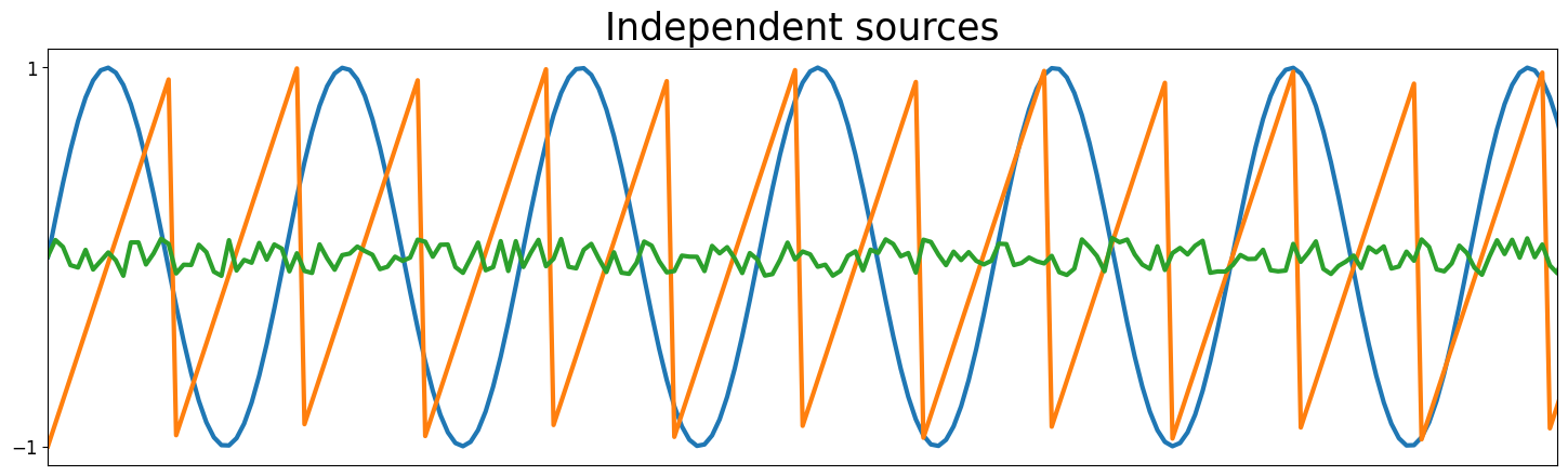
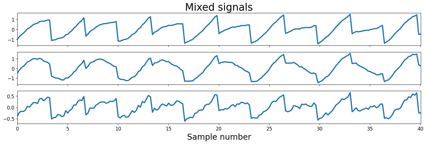
Viene generato un campione test con 200 campioni di 3 osservazioni, come risultato del mix di 3 segnali indipendenti, da ricostruire con l’algoritmo ICA.
Show code cell source
# Set a seed for the random number generator for reproducibility
np.random.seed(23)

# Number of samples
ns = np.linspace(0, 200, 1000)

noise_ampl = .2
noise_avg  = .0

# Source matrix
S = np.array([np.sin(ns * 1),
              signal.sawtooth(ns * 1.9),
              noise_ampl*( np.random.random(len(ns)) - .5) + noise_avg ]).T

# Mixing matrix
A = np.array([[0.5, 1, 0.2],
              [1, 0.5, 0.4],
              [0.5, 0.8, 1]])

# Mixed signal matrix
X = S.dot(A).T
Show code cell source
# Plot sources & signals
fig, ax = plt.subplots(1, 1, figsize=[18, 5])
ax.plot(ns, S, lw=3)
ax.set_xticks([])
ax.set_yticks([-1, 1])
ax.set_xlim(ns[0], ns[200])
ax.tick_params(labelsize=12)
ax.set_title('Independent sources', fontsize=25)

fig, ax = plt.subplots(3, 1, figsize=[18, 5], sharex=True)
ax[0].plot(ns, X[0], lw=3)
ax[0].set_title('Mixed signals', fontsize=25)
ax[0].tick_params(labelsize=12)

ax[1].plot(ns, X[1], lw=3)
ax[1].tick_params(labelsize=12)
ax[1].set_xlim(ns[0], ns[-1])

ax[2].plot(ns, X[2], lw=3)
ax[2].tick_params(labelsize=12)
ax[2].set_xlim(ns[0], ns[-1])
ax[2].set_xlabel('Sample number', fontsize=20)
ax[2].set_xlim(ns[0], ns[200])

plt.show()
22.2.4.3. Algoritmo#
22.2.4.3.1. Pre-processing#
L’osservazione \(\mathbf{X}\) vengono depurate dalla media e viene usata una trasformazione per combinare le osservazioni originali e ottenere un nuovo segnale \(\mathbf{X}_w\) con componenti non correlate. Il procedimento viene illustrato per i dati organizzati nella matrice,
in cui la colonna \(j\)-esima contiene le \(n_x\) osservazioni relative all’indice \(j\) (istante di tempo, paziente,…), mentre la riga \(i\)-esima contiene l’osservazione della quantità identificata dall’indice \(i\) per ogni valore di \(j\) (istante di tempo, paziente,…).
Teoria
Vengono svolte due operazioni:
rimozione della media dalle osservazioni di ogni quantità, quindi rimozione del valore medio di ogni riga, $\(X_{ij} \quad \leftarrow \quad X_{ij} - \frac{1}{n_s} \sum_{j = 1}^{n_s} X_{ij} \ ,\)$ in modo da avere i nuovi segnali a media nulla;
ricerca di una trasformazione di coordinate (combinazione delle osservazioni) che renda la nuove componenti non correlate. Una stima senza bias della correlazione è
\[\hat{\mathbf{R}} = \frac{1}{n_s - 1} \mathbf{X} \, \mathbf{X}^* \ .\]In generale, questa è una matrice piena di dimensioni \((n_x, n_x)\). Si vuole cercare la trasformazione di coordinate \(\mathbf{X}_w = \mathbf{W}_w \mathbf{X}\), che garantisce che la nuove osservazioni siano non correlate con varianza unitaria (come white noise, e da qui il nome whitening), cioè
\[\mathbf{I} = \hat{\mathbf{R}}_w = \frac{1}{n_s - 1} \mathbf{X}_w \, \mathbf{X}_w^* = \frac{1}{n_s - 1} \mathbf{W}_w \, \mathbf{X} \, \mathbf{X}^* \, \mathbf{W}_w^* = \mathbf{W}_w \, \hat{\mathbf{R}} \, \mathbf{W}_w^*\]E” possibile trovare la matrice desiderata \(\mathbf{W}_w\) usando una tecnica di scomposizione della matrice di correlazione \(\hat{\mathbf{R}}\), simmetrica (semi)definita positiva, come ad esempio la
scomposizione agli autovalori, \(\hat{\mathbf{R}} = \mathbf{E} \, \symbf{\Lambda} \, \mathbf{E}^{-1}\), con \(\symbf{\Lambda}\) diagonale; sfruttando le proprietà delle matrici sdp, si può scrivere \(\hat{\mathbf{R}} = \mathbf{E} \, \symbf{\Lambda} \, \mathbf{E}^*\), con la matrice \(\mathbf{E}\) ortogonale tale che \(\mathbf{E} \, \mathbf{E}^* = \mathbf{I}\).
la SVD, \(\hat{\mathbf{R}} = \mathbf{U} \symbf{\Sigma} \mathbf{V}^*\), con \(\symbf{\Sigma}\) diagonale; nel caso di matrice di partenza sdp, si può scrivere si può scrivere \(\hat{\mathbf{R}} = \mathbf{U} \symbf{\Sigma} \mathbf{U}^*\), con la matrice \(\mathbf{E}\) ortogonale tale che \(\mathbf{U} \, \mathbf{U}^* = \mathbf{I}\).
Sfruttando quindi la proprietà delle scomposizioni presentate sopra, osservando l’analogia del risultato delle due scomposizioni nel caso di matrice sdp, e definendo \(\symbf{\Sigma}^{1/2}\) la matrice diagonale con elementi le radici quadrate di \(\symbf{\Sigma}\), si può scrivere
\[\begin{split}\begin{aligned} \mathbf{I} & = \mathbf{W}_w \, \hat{\mathbf{R}} \, \mathbf{W}_w^* = \\ & = \mathbf{W}_w \, \mathbf{U} \symbf{\Sigma}^{\frac{1}{2}} \symbf{\Sigma}^{\frac{1}{2}} \mathbf{U}^* \, \mathbf{W}_w^* = \\ & = \mathbf{W}_w \, \mathbf{U} \symbf{\Sigma}^{\frac{1}{2}} \mathbf{U}^* \mathbf{U} \symbf{\Sigma}^{\frac{1}{2}} \mathbf{U}^* \, \mathbf{W}_w^* = \\ & = (\mathbf{W}_w \, \mathbf{U} \symbf{\Sigma}^{\frac{1}{2}} \mathbf{U}^* ) \, (\mathbf{W}_w \, \mathbf{U} \symbf{\Sigma}^{\frac{1}{2}} \mathbf{U}^* )^* \ , \end{aligned}\end{split}\]e quindi (todo gisutificare la comparsa di \(\mathbf{U}^* \mathbf{U}\) per ottenere una matrice quadrata, giustificare la scelta di \(\mathbf{W}_w \, \mathbf{U} \symbf{\Sigma}^{\frac{1}{2}} \mathbf{U}^* = \mathbf{I}\))
\[\mathbf{W}_w \, \mathbf{U} \symbf{\Sigma}^{\frac{1}{2}} \mathbf{U}^* = \mathbf{I} \qquad \rightarrow \qquad \mathbf{W}_w = \mathbf{U} \symbf{\Sigma}^{-\frac{1}{2}} \mathbf{U}^* \]
Show code cell source
def center(x):
    """ Remove average value """
    mean = np.mean(x, axis=1, keepdims=True)
    centered =  x - mean

    return centered, mean


def covariance(x):
    """ Evaluate signal covariance, with unbiased estimator """
    mean = np.mean(x, axis=1, keepdims=True)
    n = np.shape(x)[1] - 1
    m = x - mean

    return (m.dot(m.T))/n


def whiten(x):
    """
    Whiten signal x: find the lnear transformation provinding a trasformed uncorrelated signal
    """
     # Calculate the covariance matrix
    coVarM = covariance(X)

    # Single value decoposition
    U, S, V = np.linalg.svd(coVarM)

    # Calculate diagonal matrix of eigenvalues
    d = np.diag(1.0 / np.sqrt(S))

    # Calculate whitening matrix
    whiteM = np.dot(U, np.dot(d, U.T))

    # Project onto whitening matrix
    Xw = np.dot(whiteM, X)

    return Xw, whiteM
22.2.4.3.2. FastICA#
Viene qui illustrato l’algoritmo FastICA1
todo
def fastIca(signals,  alpha = 1, thresh=1e-8, iterations=5000):
    m, n = signals.shape

    # Initialize random weights
    W = np.random.rand(m, m)

    for c in range(m):
            w = W[c, :].copy().reshape(m, 1)
            w = w / np.sqrt((w ** 2).sum())

            i = 0
            lim = 100
            while ((lim > thresh) & (i < iterations)):

                # Dot product of weight and signal
                ws = np.dot(w.T, signals)

                # Pass w*s into contrast function g
                wg = np.tanh(ws * alpha).T

                # Pass w*s into g prime
                wg_ = (1 - np.square(np.tanh(ws))) * alpha

                # Update weights
                wNew = (signals * wg.T).mean(axis=1) - wg_.mean() * w.squeeze()

                # Decorrelate weights
                wNew = wNew - np.dot(np.dot(wNew, W[:c].T), W[:c])
                wNew = wNew / np.sqrt((wNew ** 2).sum())

                # Calculate limit condition
                lim = np.abs(np.abs((wNew * w).sum()) - 1)

                # Update weights
                w = wNew

                # Update counter
                i += 1

            W[c, :] = w.T
    return W
22.2.4.4. Applicazione del metodo al segnale#
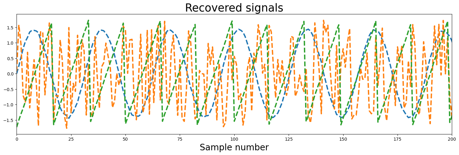
Il metodo viene applicato al problema considerato. In questo caso (segnali non gaussiani,…) il metodo riesce a ricostruire bene (todo è un bene «a occhio», qualitativo. Quantificare!) i 3 segnali indipendenti di partenza a meno di un fattore moltiplicativo, arbitrarietà propria del metodo.
todo Dire qualcosa sulle componenti principali indipendenti, discutendo le componenti della matrice \(\mathbf{W}\)
#> Preprocessing
# Center signals
Xc, meanX = center(X)

# Whiten mixed signals
Xw, whiteM = whiten(Xc)
#> FastICA
W = fastIca(Xw,  alpha=1)

#> Find unmixed signals using
unMixed = Xw.T.dot(W.T)
Show code cell source
# Plot input signals (not mixed)
fig, ax = plt.subplots(1, 1, figsize=[18, 5])
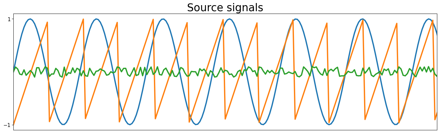
ax.plot(S, lw=3)
ax.tick_params(labelsize=12)
ax.set_xticks([])
ax.set_yticks([-1, 1])
ax.set_title('Source signals', fontsize=25)
ax.set_xlim(0, 200)
fig, ax = plt.subplots(1, 1, figsize=[18, 5])
ax.plot(unMixed, '--', label='Recovered signals', lw=3)
ax.set_xlabel('Sample number', fontsize=20)
ax.set_title('Recovered signals', fontsize=25)
ax.set_xlim(0, 200)
plt.show()
#> Comparison of matrices involved, A, whiteM, W
# todo...