11.4.4. Electromagnetic circuits#
Guidlines for solution
Find the equivalent magnetic network of the inductive part of the system to find the relation,
\[\mathbf{v}(t) = \dot{\symbf{\psi}}(t) = \frac{d}{dt} \left( \mathbf{L} \, \mathbf{i}(t) \right) \ ,\]between the tensions and the currents at the ports of the electromagnetic system, usually under the assumpsions of
no dispersed fluxes,
linear constitutive equation of the ferromagnetic medium, \(b = \mu_{\text{Fe}} h\), so that hysteresis is neglected
permeability of the ferromagnetic much larger than the permeability of free space, \(\mu_{\text{Fe}} \gg \mu_0\), so that the reluctance of the ferrmagnetic medium is negligible if compared with the reluctance of the air gaps. Relucatnce of air gaps reads
\[\theta = \frac{\delta}{\mu_0 A} \ .\]In stationary regime \(\frac{d}{dt} \equiv 0\), and thus inductors act as short-circuits.
Use the relation \(\mathbf{v} = \frac{d}{dt} \left( \mathbf{L} \, \mathbf{i} \right)\) in the electric network to solve the electromagnetic system
Find all the other physical quantities needed, remembering that the volume density of electromagnetic energy in media, under the assumption of linear media, is
\[u = \frac{1}{2 \mu} \left|\vec{b}(\vec{r},t)\right|^2 + \frac{1}{2} \varepsilon \left|\vec{e}(\vec{r},t)\right|^2 \ .\]Volume density must be integrated over the regions of space where it’s not negligible, like air gaps.
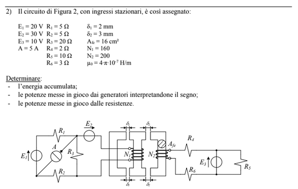
Exercise 11.15 (Exam 2025-01-22, Exercise 3.)
Solution
|
|
|
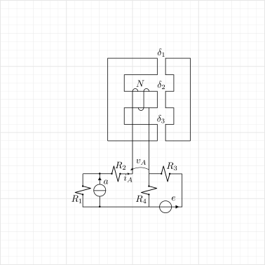
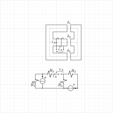
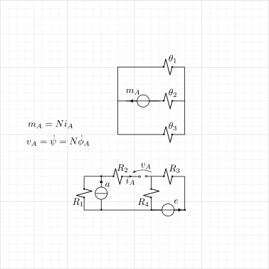
Equivalent magnetic network of the inductive part of the system. The equivalent reluctance seen by the magnetic flux generator \(m_A = N i_A\) is
\[\theta_{eq} = \theta_2 + \left( \theta_1 \parallel \theta_3 \right) \ .\]and thus the flux through it reads
\[\phi_A = \frac{m_A}{\theta_{eq}} = \frac{N}{\theta_{eq}} i = \dots\]The parallel part of the circuit acts as a current divider and thus magnetic fluxes through gaps \(1\) and \(3\) are
(11.2)#\[\begin{split}\begin{aligned} \phi_1 & = \frac{\theta_3}{\theta_1 + \theta_3} \phi_A = \frac{\theta_3}{\theta_1 + \theta_3} \frac{N}{\theta_{eq}} i_A = \dots \\ \phi_3 & = \frac{\theta_1}{\theta_1 + \theta_3} \phi_A = \frac{\theta_1}{\theta_1 + \theta_3} \frac{N}{\theta_{eq}} i_A = \dots \\ \end{aligned}\end{split}\]Faraday’s law provides the relation between the voltage and the concatenated flux,
\[v_A = \dot{\psi} = N \dot{\phi}_A = \frac{N^2}{\theta_{eq}} \dfrac{d i_A}{dt} = L_{eq} \dfrac{di}{dt} \ ,\]where the equivalent inductance of the magnetic circuit
\[L_{eq} = \dots\]has been introduced. This relation becomes \(v_A = 0\) in steady regime.
The electric network can be solved evaluating Thevenin equivalent network at the inductive port,
\[\begin{split}\begin{aligned} v_{Th} & = \frac{R_3}{R_2 + R_3} e + R_1 a \\ R_{Th} & = R_1 + R_2 + \left( R_3 \parallel R_4 \right) \ , \end{aligned}\end{split}\]Thus the KVL on the equivalent complete network is
\[v_{Th} - R_{Th} i_A - L \dfrac{d i_A}{d t} = 0 \ . \]In steady regime, \(\frac{d}{dt} \equiv 0\), and thus
(11.3)#\[\overline{i}_A = \dfrac{v_{Th}}{R_{Th}} = \dots \]Energy stored in the magnetic field is the sum (integral) of the contribution \(\frac{1}{2 \mu} \left|\vec{b}\right|^2\) in electromagnetic energy density, \(u\). With the assumption of negligible reluctance of the ferromagnetic medium,
\[\begin{split}\begin{aligned} \int_{V} \frac{1}{2 \mu} \left| \vec{b} \right|^2 & \sim \int_{V_{gaps}} \frac{1}{2 \mu_0} \left| \vec{b}(\vec{r},t) \right|^2 = \\ & \sim \sum_{k \in \text{gaps}} \frac{1}{2 \mu_0} b_k^2 \, V_k = \\ & \sim \sum_{k \in \text{gaps}} \frac{1}{2 \mu_0} \left(\frac{\phi_k}{A_k}\right)^2 \, A_k \, \delta_k = \\ & \sim \sum_{k \in \text{gaps}} \frac{1}{2} \frac{\delta_k}{\mu_0 A_k} \phi_k^2 = \\ & \sim \sum_{k \in \text{gaps}} \frac{1}{2} \theta_k \phi_k^2 = \dots \ . \end{aligned}\end{split}\]Fluxes can be evaluated with relations (11.2), once the current \(i_A\) is known, from (11.3).
After solving the electric circuit (e.g. introducing two loop currents in the left and right loops), powers through resistors and generators read
\[\begin{split}\begin{aligned} P_{R_1} & = R_1 \, i_1^2 = R_1 (i_A - a)^2 = \dots \\ P_{R_2} & = R_2 \, i_2^2 = R_2 i_A^2 = \dots \\ P_{R_3} & = R_3 \, i_3^2 = R_3 (i_A - i_{e,1})^2 = \dots \\ P_{R_4} & = R_4 \, i_4^2 = R_4 (i_A + i_{e,1})^2 = \dots \\ \end{aligned}\end{split}\]\[\begin{split}\begin{aligned} P_a & = v_a a = R_1 (i_A-a) \, a = \dots \\ P_e & = e i_e = e ( -i_A + i_{e,1} ) = \dots \\ \end{aligned}\end{split}\]with \(i_{e,1} = \frac{e}{R_3 + R_4}\).
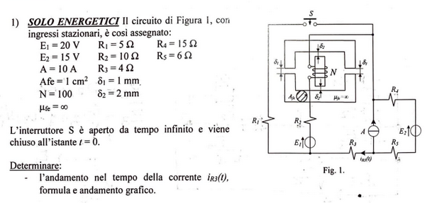
Exercise 11.16 (Exam 2024-06-19, Exercise 2.)
Solution - todo
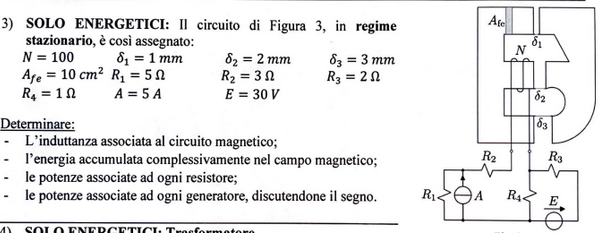
Exercise 11.17 (Exam 2024-02-13, Exercise 1a.)