11. Rebalancing#
While investing should not be confused with gambling, some games, gambling and betting strategies could provide useful toy-problems and introduction to investing principles. This is the case of gambling on a coin flip game that is discussed here and used to introduce the concept of rebalancing.
Rebalancing:
reduces the dispersion of the composite return
improves risk-adjusted return
may also improve the expected value of the composite return as well (rebalancing premium, or Shannon’s demon), for processes that meet some particular conditions
Contents
11.1. Example: coin flip game#
In this section, the effect of rebalancing is discussed in a coin flip game. This game can be interpreted as a very simple model of a 2-asset portfolio, with 1 risky asset with only two outcomes (win or loss), and 1 safe asset (no real return).
Example 11.1 (Shannon demon in a coin flip game)
Starting with \(100 \text{€}\), and a fair coin with \(50\%\) probability of for each outcome, either \(\text{H: head}\) or \(\text{T: tail}\). If outcome is \(\text{H}\) you gain \(50\%\), if the outcome is \(\text{T}\) you lose \(33.3\%\).
Let’s evaluate two different strategies:
play with all the money you have
at every toss, bet \(50\%\) of the amount you have
What’s the expected amount at the end of the game? What’s the amount distribution? …
Here the problem is investigated for a set of different strategies uniquely determined by different values of the betting fraction \(f\).
As discussed below, the optimal fraction (optimal in the sense of maximum expected geometric return; but does this definition of optimum meet your taste — e.g. your risk tolerance to negative results and dispersion of the results?) is
Show code cell source
#> Reset variables
%reset -f
Show code cell source
# -----------------------------------------------------------------------------
# - Import libraries
# - model single coin event: Bernoulli distribution (here choice) and gain/loss
# - number of consecutive tosses per realization, number of realizations
# -----------------------------------------------------------------------------

#> Libraries
import numpy as np
import matplotlib.pyplot as plt

#> Coin toss as a Bernoulli random variable
fracs = [ .0, .2, .4, .6, .8, 1.]
colors = plt.cm.tab10.colors
n_fracs = len(fracs)
# frac = .2

#> Bernoulli distribution
# X = 0 (loss)   p(0) = 1 - p
#     1 (win)    p(1) = p
p_win = .5      # probability of win ( 0 <= p_win <= 1 )
p_los = 1. - p_win

#> Gain and loss
# here outcome_loss is defined as negative number, while in the text is defined
# as a positive number. Nothing changes: just take the inverse of l -> -l
outcome_gain, outcome_loss = .5, -1./3.

#> N.of coin toss and realizations
n_tosses = 30
n_reals = 2000
Show code cell source
# -----------------------------------------------------------------------------
# Check Kelly criterion, see below
# -----------------------------------------------------------------------------
frac_opt = p_win / np.abs(outcome_loss) - p_los / outcome_gain

print(f"Kelly criterion, optimal fraction f*")
print(f"frac_opt: {frac_opt}")
Show code cell output
Kelly criterion, optimal fraction f*
frac_opt: 0.5
Show code cell source
# -----------------------------------------------------------------------------
# Test strategies for different values of f
# -----------------------------------------------------------------------------

#> Random number generator
rng = np.random.default_rng().choice
rng_params = {'a': [outcome_gain, outcome_loss], 'p': [p_win, p_los], 'size': n_tosses}

trials = []

#> Test different strategies, with different value of frac
for frac in fracs:

    w_mat = []
    for real in np.arange(n_reals):

        outcomes = np.array( [0] + list(rng(**rng_params)) )
        w_mat += [ np.cumprod(1+frac*outcomes) ]

    w_mat = np.array(w_mat).T

    trial = { 'f': frac, 'w': w_mat }
    trials += [ trial ]
Show code cell source
# -----------------------------------------------------------------------------
# Results and plots
# -----------------------------------------------------------------------------
#> Distribution of outcomes
fig, ax = plt.subplots(len(fracs),4, figsize=(10,6))
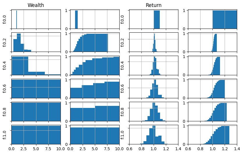
print("fraction, avg wealth, avg geo return, n.negative outcomes")
for itrial in np.arange(n_fracs):
w_avg = np.mean(trials[itrial]['w'][-1,:])
r_end = trials[itrial]['w'][-1,:]**(1/n_tosses)
r_avg = np.mean(r_end)
n_neg = np.sum(trials[itrial]['w'][-1,:] < 1.)
print(f"f:{fracs[itrial]}, w_avg:{w_avg:6.3f}, r_avg:{r_avg:6.3f}, n_neg:{n_neg:4d}")
ax[itrial,0].hist(trials[itrial]['w'][-1,:], density=True,) # , histtype='step', linewidth=1.5, alpha=.7
ax[itrial,0].set_xlim(0,10)
ax[itrial,1].hist(trials[itrial]['w'][-1,:], bins=100, density=True, cumulative=True)
ax[itrial,1].set_xlim(0,10)
if ( not itrial == n_fracs-1):
ax[itrial,0].set_xticklabels([])
ax[itrial,1].set_xticklabels([])
ax[itrial,0].set_yticklabels([])
ax[itrial,0].set_ylabel(f"f:{fracs[itrial]}")
ax[itrial,0].grid(); ax[itrial,1].grid()
ax[itrial,2].hist(r_end, density=True,) # , histtype='step', linewidth=1.5, alpha=.7
ax[itrial,2].set_xlim(0.6, 1.4)
ax[itrial,3].hist(r_end, bins=100, density=True, cumulative=True)
ax[itrial,3].set_xlim(0.6, 1.4)
if ( not itrial == n_fracs-1):
ax[itrial,2].set_xticklabels([])
ax[itrial,3].set_xticklabels([])
ax[itrial,2].set_yticklabels([])
ax[itrial,2].set_ylabel(f"f:{fracs[itrial]}")
ax[itrial,2].grid(); ax[itrial,3].grid()
if ( itrial == 0 ):
ax[itrial,0].set_title("Wealth")
ax[itrial,2].set_title("Return")
fraction, avg wealth, avg geo return, n.negative outcomes
f:0.0, w_avg: 1.000, r_avg: 1.000, n_neg:   0
f:0.2, w_avg: 1.640, r_avg: 1.013, n_neg: 356
f:0.4, w_avg: 2.715, r_avg: 1.021, n_neg: 571
f:0.6, w_avg: 4.588, r_avg: 1.022, n_neg: 551
f:0.8, w_avg: 6.172, r_avg: 1.014, n_neg: 871
f:1.0, w_avg: 9.417, r_avg: 1.002, n_neg: 857
todo
Improve plot quality: very poor \(\texttt{hist}\) outcome
Discuss:
difference between algebraic and geometric return (compounding)
probability of negative outcomes and dispersion of the results
probability of intermediate negative outcomes and dispersion of results (time effect and volatility)
comparison with no-rebalancing strategy
Show code cell source
# #> History of the
# fig, ax = plt.subplots(1,1)
# ntrials = len(trials)
# for itrial in np.arange(ntrials):
#   trial = trials[itrial]
#   ax.semilogy(trial['w'], lw=.2, alpha=.5, color=colors[itrial])
# ax.grid()
Example 11.2 (Interludio: is the coin fair?)
After tossing a coin \(10\) times and getting \(10\) Heads in a row, would you bet on Head or Tail?
Although every toss is a statistically independent event, a very unlikely series of outcomes under the assumption of a fair coin may induce some doubts about the truthfulness of this assumption.
See here: Inferential statistics - Hypotesis testing (Fisher) - Is the coin fair? as an example. If you want to play a bit with the notebook, just open it in Colab: the script is originally meant for \(n=30\) coin flips; just 1) set \(\texttt{n\_flips = 10}\); 2) run it again; 3) get the value of the extreme event proabability (either \(10\) Heads or \(10\) Tails) to address the question of the interludio,
i.e. the probability of getting \(10\) consecutive outcomes in the first \(10\) flips with a fair coin is less than \(0.1\%\). A pretty low probability that the null hypotesis “the coin is fair” holds…
Here for the application of Fisher criterion for hypotesis testing for two coins with \((p_H, p_T)^{1} = (0.5, 0.5)\) and \((p_H, p_T)^{2} = (0.45, 0.55)\).
Example 11.3 (Kelly criterion for the coin flip game)
Let \(p\) the probability of a win, \(q = 1-p\) the probability of a loss, \(g\) is the net fraction gained in a win, \(l\) is the net fraction lost in a loss. The strategy is simple: always bet the fraction \(f\) of the amount you have. Is there an optimal value \(f^*\) that maximizes the expected return?
todo Clean this section containing mathematical details about Kelly’s criterion.
Amount after \(\, n \, \) coin tosses
Geometric return
Optimization of the expecte value of the geometric return
free or constrained optimization,…
Starting with the amount \(x_0\), the expected amount after 1 toss reads
while the actual amount,
the amount after 1 coin toss is a random variable depending on the result of the toss, represented by a \(X_1 \in \{0, 1\}\) of the coin toss, \(\text{0: loss}\), \(\text{1: win}\), reads
After the second toss,
and after the \(n^{th}\) toss
The maximization of the \(\ln \frac{x_n}{x_0}\) (equivalent to the maximization of \(\frac{x_n}{x_0}\)),
w.r.t. \(f\) gives
The expected value of the logarithm of the ratio reads
and its derivative w.r.t. \(f\) reads
and becomes zero (so that \(\mathbb{E}[ x_n ]= x_0\) and return is zero) when
and
Is this an maximum? Compute the second-order derivative \(\dfrac{d^2}{df^2} \mathbb{E}\left[ \ln \frac{x_n}{x_0} \right]\), evaluate it in \(f^*\) and check if it’s \(< 0\). By direct computation, the second order derivative
is always negative for \(p \in [0,1]\), i.e. for all the possible values of the win probability of the probability distribution. Thus, the extreme point found above is a maximum.
First order derivative for \(f = 0\).
The condition for the first derivative in \(f=0\) to be positive is equivalent to the condition of \(f^* > 0\), i.e. optimal fraction is feasible, \(f^* \in [0,1]\).
Is this maximum feasible? If no short (betting against, \(f \ge 0\)) and no leverage (betting more than you have, \(f \le 1\)) betting is possible, the fraction \(f\) must lie in range \([0,1]\): the maximization problem is not a free optimization problem, but a simple constrained optimization problem. In these problems — under the assumptions of sufficient regularity of the function — extreme points may occur where first order derivative is zero or at the boundary of the domain.
Thus:
either the maximum is at \(f^*\), if \(f^* \in [0,1]\), \(0 \le p(l+g) - l \le lg\)
or the maximum is at \(f^* = 0\): the probability is against you, so you’d better do nothing
or the maximum is at \(f^* = 1\): the probability is with you, so you’d better bet (if your risk tolerance accepts the dispersion of the results)
If short is allowed, there’s no constraint \(f \ge 0\); if leverage betting is allowed, there’s no constraint \(f \le 1\).
What’s the optimal expected value? Evaluate \(\mathbb{E}\left[ \ln \frac{x_n}{x_0} \right]\left( f^* \right)\)