20. Rebalancing

In this Notwbook, two strategies on a 2-asset portfolio are discussed and compared:

• rebalanced portfolio, after each period

• buy-and-hold portfolio, without rebalancing

Effects of rebalancing and conditions for rebalancing premium are discussed: sometimes the expected log-return of the rebalanced portfolio may exceed the expected log-return of each single asset.

20.1. Libraries, parameters and useful functions

Libraries are imported and useful functions to treat conics below are defined here

20.1.1. Libraries

Show code cell content Hide code cell content

import numpy as np
import matplotlib.pyplot as plt
from ipywidgets import interact, FloatSlider

20.1.2. Parameters

Show code cell content Hide code cell content

#>
params = {
    '2-asset-portfolio': { 'mu1': .10, 'sigma1': .20, 'mu2': .08, 'sigma2': .15, 'rho': -.25}
}

20.1.3. Functions for conics

Show code cell content Hide code cell content

def conics_points(a,b,c,d,e,f,n=100,printout=False):
    """  ax^2 + bxy + cy^2 + dx + ey + f = 0  """
    delta = b**2 - 4*a*c
    if delta == 0.:   # possible parabola (comparison with reals?)
        ctype = 'parabola'
        x,y = np.zeros(n+1)
    elif delta < 0.:  # possible ellipse
        ctype = 'ellipse'
        x,y = ellipse_points(a,b,c,d,e,f,n,printout)
    else:             # possible hyperbola
        ctype = 'hyperbola'
        x,y = np.zeros(n+1)

    return ctype, x, y

def ellipse_points(a,b,c,d,e,f,n=100,printout=False):
    """  """
    theta = np.pi / 4. * ( a == c ) + .5 * np.arctan2(b,a-c) * ( not a == c )
    if printout: print(f"theta: {theta}")
    A = a * ( np.cos(theta) )**2 + b * np.cos(theta) * np.sin(theta) + c * ( np.sin(theta) )**2
    B = ( c - a ) * np.sin(2*theta) + b * np.cos(2*theta)
    C = a * ( np.sin(theta) )**2 - b * np.cos(theta) * np.sin(theta) + c * ( np.cos(theta) )**2
    D =  d * np.cos(theta) + e * np.sin(theta)
    E = -d * np.sin(theta) + e * np.cos(theta)
    F = f

    if ( A < 0 and C < 0 ):
        A = -A; B = -B; C = -C; D = -D; E = -E; F = -F
    elif ( A == 0 )  :  raise ValueError("A = 0")
    elif ( C == 0 )  :  raise ValueError("C = 0")
    elif ( A*C < 0. ):  raise ValueError(f"A*C={A*C} <= 0")

    uc = - .5 * D / A
    vc = - .5 * E / C
    FF = A * uc**2 + C * vc**2 - F

    if printout: print(f"uc: {uc}\nvc: {vc}\nFF: {FF}")

    if FF > 0:
        if printout: print(f"A: {A}\nB: {B}\nC: {C}\nD: {D}\nE: {E}\nF: {F}")

        semi_a = np.sqrt(FF/A)
        semi_b = np.sqrt(FF/C)

        if printout: print(f"semi_a: {semi_a}\nsemi_b: {semi_b}")

        thv = np.linspace(0, 2*np.pi, n+1);  thv[-1] = thv[0]

        u, v = semi_a * np.cos(thv), semi_b * np.sin(thv)
        x = ( u + uc ) * np.cos(theta) - ( v + vc ) * np.sin(theta)
        y = ( u + uc ) * np.sin(theta) + ( v + vc ) * np.cos(theta)

        return x,y

    else:
        raise ValueError(f"FF:{FF} <= 0")

    # else: 0: degenerate ellipse; <0: not an ellipse! (what's that?)

20.2. Rebalanced portfolio

Let the 1-period return of the assets be normal (todo is this necessary? Can’t one rely on central limit theorem? How long the summation must be for convergence to normal distribution, in presence of heavy-tails distribution? If one can’t rely on central limit theorem, let use numerical methods to investigate the effect of heavy tails distributions),

\[\mathbf{r} \sim \mathscr{N} \left( \boldsymbol{\mu}, \boldsymbol{\sigma}^2 \right) \ .\]

Compound return of the portfolio has expected value

\[\mu^c_p = \mathbb{E}[r^c_p] = \mathbf{w}^T \boldsymbol{\mu} - \dfrac{1}{2}\mathbf{w}^T \boldsymbol{\sigma}^2 \, \mathbf{w}\]

and variance

\[\begin{aligned} \sigma_{r^c_p}^2 & = \mathbb{E}\left[(r^c_p - \mu^c_p )^2 \right] = \dots = \mathbf{w}^T \boldsymbol{\sigma} \mathbf{w} \end{aligned}\]

20.2.1. Shannon demon

Sometimes the expected value of the compound return of the rebalanced portfolio can be larger than the expected return of each asset class.

\[\mu^c_k = \mathbb{E}[r^c_k] = \mu_k - \dfrac{\sigma_k^2}{2}\]

Example: 2-asset portfolio. As an example, the expected value of the compund return of a 2-asset rebalanced portfolio,

\[\mathbb{E} [ r_p^c ] = w_1 \mu_1 + w_2 \mu_2 - \dfrac{1}{2} ( w_1^2 \sigma_1^2 + 2 w_1 w_2 \rho \sigma_1 \sigma_2 + w_2^2 \sigma_2^2 )\]

Using \(w_1\), \(w_2\) as independent variables, for any value of the expected return, the expression of the return itself can be represented as a conic section in the \(w_1,w_2\)-plane. In particular,

• for \(\rho \ne 1\), it’s an ellipse (\(\Delta = B^2 - 4 A C < 0\)),

• for \(\rho = 1\), it’s a parabola (\(\Delta = 0\))

Portfolio allocation. Some constraints may hold on portfolio allocation:

• fully-invested: \(w_1 + w_2 = 1\)

• no short-selling: \(w_1,\ w_2 \ge 0\)

• no leverage: \(w_1, \ w_2 \le 1\)

Show code cell source Hide code cell source

def plot_shannon_demon_set(rho, mu1, sigma1, mu2, sigma2):
    #> Plot parameters
    xmin, xmax, nx = -10.5, 11.5, 21
    ymin, ymax, ny = -10.5, 11.5, 21

    #> Expected value of single-asset compound returns
    ElnP1 = mu1 - .5 * sigma1**2
    ElnP2 = mu2 - .5 * sigma2**2

    ElnP = max(ElnP1, ElnP2)     # Take max for comparison

    #> Define conics coefficients and find points
    a, b, c, d, e, f = -.5*sigma1**2, -rho*sigma1*sigma2, -.5*sigma2**2, mu1 ,mu2, -ElnP
    ctype, x, y = conics_points(a,b,c,d,e,f, printout=False)

    #> Plot
    print(f"max(ElnP1, ElnP2): {ElnP}")

    fig, ax = plt.subplots(1,1, figsize=(5,5))
    ax.plot(x,y)
    ax.fill(x,y, alpha=.3)
    ax.plot(np.linspace(0,1), np.linspace(1,0), color='black')
    ax.grid()
    ax.set_aspect('equal') # , 'box')
    ax.set_xlim(-.5,1.5)
    ax.set_ylim(-.5,1.5)
    ax.set_xlabel("$w_1$")
    ax.set_ylabel("$w_2$")

#> Initial value of params
mu1    = params['2-asset-portfolio']['mu1']
sigma1 = params['2-asset-portfolio']['sigma1']
mu2    = params['2-asset-portfolio']['mu2']
sigma2 = params['2-asset-portfolio']['sigma2']
rho    = params['2-asset-portfolio']['rho']

#> Interactive plot
interact(
    plot_shannon_demon_set,
    rho=FloatSlider(   value=rho   , min=-1.0 , max=1.0, step=0.01, description='rho'),
    mu1=FloatSlider(   value=mu1   , min=-0.30, max=.30, step=0.01, description=f'mu1'),
    mu2=FloatSlider(   value=mu2   , min=-0.30, max=.30, step=0.01, description=f'mu2'),
    sigma1=FloatSlider(value=sigma1, min= .0  , max=.30, step=0.01, description=f'sig1'),
    sigma2=FloatSlider(value=sigma2, min= .0  , max=.30, step=0.01, description=f'sig2')
);

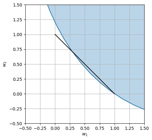
This plot represents in blue asset allocations of the balanced 2-asset portfolio with expected value of the compound return larger than the compound return of any individual asset. Black line represents all the possible allocations of a fully invested portfolio, \(w_1+w_2=1\) with no leaverage \(w_k \le 1\) and not short selling \(w_k \ge 0\).

20.3. Comparison of portfolios: realizations of stochastic processes

In this section, rebalanced portfolio and buy-and-hold portfolio are compared. Different realizations of these two portfolio strategies are built, and used to build statistics, and discuss their properties in terms of compound return, drawdowns,…

Note. Here, 1-period returns are modelled as normal random variable so far. Anyways, it’s possible (and suggested) to implement the most suited random process for modelling the return of the desired assets.

20.3.1. Useful functions

A useful function is introduced here to build correlated random variables with the desired expected values and covariance.

Main Colab notebook can be found here: https://colab.research.google.com/drive/1n5py0Zf8i3_jrTTk0AR7Noq2kBYwpaqx?authuser=1#scrollTo=gmbjbprjCHto

Show code cell content Hide code cell content

def correlated_variable_coeffs(mux, muy, sigmax, sigmay, rhoxy):
  if ( np.abs(rhoxy) > 1. ):
      raise ValueError('Invalid correlation coefficient, |rhoxy|=|{rhoxy}| > 1.')
  elif ( not rhoxy == 1. ):
      a = rhoxy * sigmay / sigmax
      sigmaz = 1.
      b = np.sqrt(sigmay**2 - a**2 * sigmax**2) / sigmaz**2
      c = 0.
      muz = (muy - c - mux * rhoxy * sigmay / sigmax) / b
  else:
      a = rhoxy * sigmay / sigmax
      muz = 0.
      sigmaz = 1.
      b = 0.
      c = muy - mux * rhoxy * sigmay / sigmax

  return muz, sigmaz, a, b, c

20.3.2. Realizations

Show code cell source Hide code cell source

#> Parameters of the 2 assets
mu1    = params['2-asset-portfolio']['mu1']      #
sigma1 = params['2-asset-portfolio']['sigma1']   #
mu2    = params['2-asset-portfolio']['mu2']      #
sigma2 = params['2-asset-portfolio']['sigma2']   #
rho    = -.5 # params['2-asset-portfolio']['rho']      #

#> Evaluate the parameters of an independent r.v. Z to build the r.v. of asset 2
# with desired average value, variance and covariance with X
muz, sigmaz, a,b,c = correlated_variable_coeffs(mu1, mu2, sigma1, sigma2, rho)

#> Weights of the 2 assets
# rebalanced ptf  : constant weights
# buy-and-hold ptf: initial weights
w1, w2 = 0.5, 0.5

#> Initial conditions
y0 = 1

#> Random number generator, representing 1-period return R_n = Y_{n}/Y_{n-1}
nreal = 1000       # n. of realizations of the random process
nt = 100           # n. of periods (toss) for each realization
tv = np.arange(nt)

#> Random number generators of the 2 assets
rng1 = np.random.default_rng().normal
rng1_params = {'loc': mu1, 'scale': sigma1, 'size': nt}

rngZ = np.random.default_rng().normal
rngZ_params = {'loc': muz, 'scale': sigmaz, 'size': nt}

#> End values, max drawdowns
y_reb_end, y_bah_end = np.zeros(nreal), np.zeros(nreal)
reb_max_drawdown, bah_max_drawdown = np.zeros(nreal), np.zeros(nreal)


fig, ax = plt.subplots(1,2, figsize=(10,5))
for ireal in np.arange(nreal):

    #> 1-period returns of the 2 assets
    r1 = rng1(**rng1_params)
    rZ = rngZ(**rngZ_params)
    r2 = a*r1 + b*rZ + c

    #> Rebalanced portfolio
    y_reb = np.zeros(nt);  y_reb[0] = y0
    y_reb[1:] = y_reb[0]*np.cumprod(1 + w1*r1[1:] + w2*r2[1:])

    #> Buy-and-hold portfolio
    y_bah_1 = np.zeros(nt);  y_bah_1[0] = y0 * w1
    y_bah_2 = np.zeros(nt);  y_bah_2[0] = y0 * w2
    y_bah_1[1:] = y_bah_1[0]*np.cumprod(1+r1[1:])
    y_bah_2[1:] = y_bah_2[0]*np.cumprod(1+r2[1:])

    y_bah = y_bah_1 + y_bah_2

    #> End values
    y_reb_end[ireal] = y_reb[-1]/y0
    y_bah_end[ireal] = y_bah[-1]/y0

    #> Max drawdowns
    y_reb_max = np.maximum.accumulate(y_reb)
    y_bah_max = np.maximum.accumulate(y_bah)

    reb_drawdowns = 1. - y_reb/y_reb_max
    bah_drawdowns = 1. - y_bah/y_bah_max

    #> Update stored realization with max drawdown
    if np.max(reb_drawdowns) > np.max(reb_max_drawdown):
        y_reb_max_drawdown = y_reb.copy()
    if np.max(bah_drawdowns) > np.max(bah_max_drawdown):
        y_bah_max_drawdown = y_bah.copy()

    reb_max_drawdown[ireal] = np.max(reb_drawdowns)
    bah_max_drawdown[ireal] = np.max(bah_drawdowns)

    if ( ireal % 10 == 0 ):
        ax[0].semilogy(tv, y_reb/y_reb[0], lw=.2, color=plt.cm.tab10.colors[0])
        ax[0].semilogy(tv, y_bah/y_bah[0], lw=.2, color=plt.cm.tab10.colors[1])

        ax[1].plot(tv, ((y_reb)/y_reb[0])**(1/(tv+1)), lw=.1, color=plt.cm.tab10.colors[0])
        ax[1].plot(tv, ((y_bah)/y_bah[0])**(1/(tv+1)), lw=.1, color=plt.cm.tab10.colors[1])

ax[0].set_ylabel("Y[n]/Y[0]")
ax[0].set_xlabel("Periods")
ax[0].grid()

ax[1].set_ylabel("Composite returns")
ax[1].set_xlabel("Periods")
ax[1].grid()



ax[0].semilogy(tv, y_reb_max_drawdown/y_reb[0], lw=1, color=plt.cm.tab10.colors[0], label='Rebalanced')
ax[0].semilogy(tv, y_bah_max_drawdown/y_reb[0], lw=1, color=plt.cm.tab10.colors[1], label='Buy-and-hold')
ax[1].plot(tv, (y_reb_max_drawdown/y_reb[0])**(1/(tv+1)), lw=1, color=plt.cm.tab10.colors[0], label='Rebalanced')
ax[1].plot(tv, (y_bah_max_drawdown/y_reb[0])**(1/(tv+1)), lw=1, color=plt.cm.tab10.colors[1], label='Buy-and-hold')


#> Analytical solution
# logret = expected_logret_fun(b,a,p,f)
# ax.semilogy(tv, y0*np.exp(logret)**tv, lw=1, color=plt.cm.tab10.colors[0])
# ax.set_ylabel("Y[n]/Y[0]")
# ax.set_xlabel("Periods")
# ax.grid()

[<matplotlib.lines.Line2D at 0x7f825f3f6fa0>]

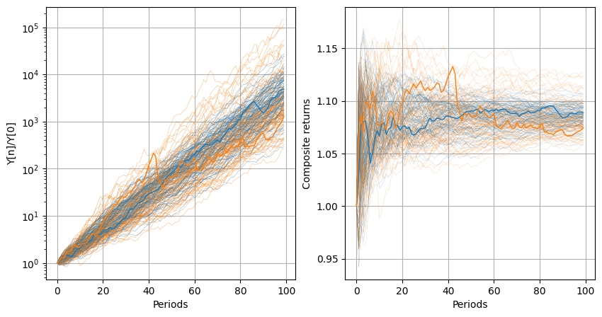
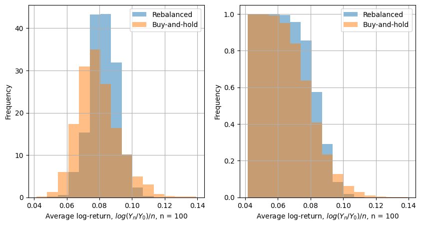
20.3.3. Composite return

Show code cell source Hide code cell source

#> Average and variance of composite return
print("Rebalanced portfolio. Compsite return")
print(f" Exp. value: {np.mean((y_reb_end/y0)**(1/nt)-1):.3f}")
print(f" Std. dev. : {np.std( (y_reb_end/y0)**(1/nt)-1):.3f}")
print("Buy-and-Hold portfolio. Compsite return")
print(f" Exp. value: {np.mean((y_bah_end/y0)**(1/nt)-1):.3f}")
print(f" Std. dev. : {np.std( (y_bah_end/y0)**(1/nt)-1):.3f}")


fig, ax = plt.subplots(1,2, figsize=(10,5))
#> Define hist bins
min_logret = min(np.min(np.log(y_reb_end/y0)/nt), np.min(np.log(y_bah_end/y0)/nt))
max_logret = max(np.max(np.log(y_reb_end/y0)/nt), np.max(np.log(y_bah_end/y0)/nt))
nbins = 15
min_bins = min_logret - (max_logret - min_logret)/nbins
max_bins = max_logret + (max_logret - min_logret)/nbins
bins = np.linspace(min_bins, max_bins, nbins+1)

#> Loop over density and cumulative probability
cum_v = [False, -1]
for i in range(2):
    ax[i].hist(np.log(y_reb_end/y0)/nt, bins=bins, density=True, cumulative=cum_v[i], alpha=.5, label="Rebalanced")
    ax[i].hist(np.log(y_bah_end/y0)/nt, bins=bins, density=True, cumulative=cum_v[i], alpha=.5, label="Buy-and-hold")
    ax[i].set_xlabel(f"Average log-return, $log(Y_n/Y_0)/n$, n = {nt}")
    ax[i].set_ylabel("Frequency")
    ax[i].legend();  ax[i].grid()

Rebalanced portfolio. Compsite return
 Exp. value: 0.086
 Std. dev. : 0.009
Buy-and-Hold portfolio. Compsite return
 Exp. value: 0.083
 Std. dev. : 0.014

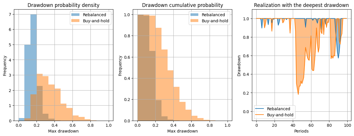
20.3.4. Maximum drawdown

Show code cell source Hide code cell source

fig, ax = plt.subplots(1,3, figsize=(15,5))
#> Define hist bins
# min_drawdown = min(np.min(y_reb_max_drawdown), np.min(y_bah_max_drawdown))
# max_drawdown = min(np.max(y_reb_max_drawdown), np.max(y_bah_max_drawdown))
nbins = 15
min_bins = 0.  # min_drawdown - (max_drawdown - min_drawdown)/nbins
max_bins = 1.  # max_drawdown + (max_drawdown - min_drawdown)/nbins
bins = np.linspace(min_bins, max_bins, nbins+1)
cum_v = [False, -1]
for i in range(2):
    ax[i].hist(reb_max_drawdown, bins=bins, alpha=.5, density=True, cumulative=cum_v[i], label="Rebalanced")
    ax[i].hist(bah_max_drawdown, bins=bins, alpha=.5, density=True, cumulative=cum_v[i], label="Buy-and-hold")
    ax[i].set_xlabel(f"Max drawdown")
    ax[i].set_ylabel("Frequency")
    ax[i].legend();  ax[i].grid()

#> Drawdowns as a function of time for the realization with deepest drawdown
reb_running_max = np.maximum.accumulate(y_reb_max_drawdown)
bah_running_max = np.maximum.accumulate(y_bah_max_drawdown)

ddown_reb = 1. - y_reb_max_drawdown/reb_running_max
ddown_bah = 1. - y_bah_max_drawdown/bah_running_max

ax[2].plot(tv, 1.-ddown_reb, color=plt.cm.tab10.colors[0], label='Rebalanced')
ax[2].plot(tv, 1.-ddown_bah, color=plt.cm.tab10.colors[1], label='Buy-and-hold')
ax[2].fill_between(tv, 1.-ddown_reb, np.ones(nt), color=plt.cm.tab10.colors[0], alpha=.5)
ax[2].fill_between(tv, 1.-ddown_bah, np.ones(nt), color=plt.cm.tab10.colors[1], alpha=.5)
ax[2].set_xlabel("Periods")
ax[2].set_ylabel("Drawdown")
ax[2].set_ylim(-.1, 1.1)
ax[2].legend()
ax[2].grid()


ax[0].set_title("Drawdown probability density")
ax[1].set_title("Drawdown cumulative probability")
ax[2].set_title("Realization with the deepest drawdown")

Text(0.5, 1.0, 'Realization with the deepest drawdown')