10. Principles of investing

10.1. Return

Return is the reward for investing. It can come from capital gain (price increase of assets bought), or periodic cashflows, like interest (from bonds), or dividends (from stocks). Some assets produce predictable return (either nominal, or real), other assets have less predictable returns. Any asset has some level of uncertainty, or risk1.

Most returns are quoted on a per-period basis - usually annually - and expressed as the percentage of the reward over the initial amount of the investment.

For a many-year investment, single-period returns compound over time.

10.1.1. Costs

While return are uncertain, at least to a certain level, usually costs - fees, expenses, taxes - or part of them, are certain. With equal other conditions, the intelligent investor should reduce costs (known), as higher costs reduce returns w/o changing the level of risk.

10.2. Risk

Risk measures uncertainty and its effects, combining probability of events and consequences of specific events. All the assets have some systematic and some specific risks .

Key measures (should give info about magnitude, frequency/probability, and duration) include:

• standard deviation or volatility: how much returns may deviate from their expected value),

• max loss (usually 100% can’t be neglected for catastrophic although rare events), value at risk (VaR, max loss with a given probability), drawdown (maximum peak-to-trough loss)

• time-to-recover (time to recover drawdowns, in a temporal perspective)

Usually, risk metrics measure uncertainty, without discerning from positive and negative events: these metrics perceive a higher-than-expected return as a risk as well. Some metrics instead, see Sortino ratio in risk-return section, aims at quantifying only negative events as risk.

10.3. Risk-Return Trade Off

“There’s no free lunch”

Higher expected returns usually come with higher risk.

…but high risk doesn’t imply high expected return

Very stupid actions usually implies poor return with high risk. Just as an example, playing Russian roulette for fun implies an expected return worse than an alternative “do-nothing and have an ice-cream instead” scenario (at least, if your goal is not to kill yourself, and your return function does not positively weight this outcome) with higher uncertainty on the final status of your health.

Sometimes the same could happen if one plays doing trading with some random meme-stocks or shit-coins.

Risk-adjusted return provides an indication of the expected return per unit of risk. Common metrics are:

• Sharpe ratio, comparing excess return and volatility compared with a “risk-free” asset - or a benchmark

  \[S := \dfrac{\mathbb{E}[R-R_b]}{\sqrt{\text{var}[R-R_b]}}\]

• Sortino ratio

  \[So := \dfrac{\mathbb{E}[R] - T}{\text{DR}} \ ,\]

  with \(T\) target return, and \(\text{DR}\) the downside deviation, i.e. the deviation w.r.t the target return evaluated only for returns \(r\) lower than the target return \(T\)

  \[\text{DR}^2 = \int_{r=-\infty}^{T} (T-r)^2 \, f(r) \, dr \ ,\]

  being \(f(r)\) the probability density function of the (continuous) random variable \(R\) representing return

10.4. Diversification

Diversification spreads risk across different investments so no single event can ruin your portfolio. Diversification works well with assets that are not - or at least they’re loosely - correlated: in this case, diversification could increase return per unit of risk.

10.5. Portfolio Construction

10.6. Time

10.6.1. Compound Return

Return of multi-period investment compounds and not simply sums. Return \(r_n\) in the \(n^{th}\) period from \(n\) to \(n+1\), is defined as

\[x_{n+1} = x_n ( 1 + r_n ) \ .\]

Over \(N\) periods, the final wealth \(x_N\) can be written as a function of the initial wealth and the 1-year returns \(r_n\),

\[x_{N} = x_0 \prod_{n=1}^N ( 1 + r_n ) \ .\]

Geometric mean provides by definition the value of the average — constant — return, \(\overline{r}\)

\[x_{N} = x_0 \prod_{n=1}^N \left( 1 + \overline{r} \right) = x_0 \left( 1 + \overline{r} \right)^N \ ,\]

and thus

\[\overline{r} = \left( \dfrac{x_N}{x_0} \right)^{\frac{1}{N}} - 1 = \left( \prod_{n=1}^N \left( 1 + r_n \right) \right)^{\frac{1}{N}} - 1 \ .\]

Logaritmic return. By the very definition of the exponential function

\[\begin{split}\begin{aligned} \ln \left( \overline{r} + 1 \right) & = \ln \left\{ \left( \prod_{n=1}^N \left( 1 + r_n \right) \right)^{\frac{1}{N}} \right\} = \\ & = \frac{1}{N} \sum_{n=1}^{N} \ln \left( 1 + r_n \right) \end{aligned}\end{split}\]

While \(\ln( 1 + r_n )\) is not Gaussian even if \(r_n\) is Gaussian, under the assumptions of the central limit theorem,

\[\ln\left( \overline{r} + 1 \right) \rightarrow \mathscr{N} \left( \mu_{\ln}, \frac{\sigma^2_{\ln}}{N} \right) \ ,\]

being \(\mu_{\ln}\) and \(\sigma^2_{\ln}\) the expected value and the variance of the i.i.d. random variables \(\ln ( 1 + r_n )\). Given the probability density \(p(r)\) of the 1-period return \(r\), these values read

\[\begin{split}\begin{aligned} \mu_{\ln} & = \int_{r} p(r) \ln ( 1 + r ) \, dr \\ \sigma_{\ln}^2 & = \int_{r} p(r) \left( \ln( 1 + r ) - \mu_{\ln} \right)^2 \, dr \ . \end{aligned}\end{split}\]

For “sufficiently small” values of \(\overline{r}\), the first-order expansion \(x \sim \ln(1+x)\), for \(x \rightarrow 0\), provides a good approximation relating the logarithmic return and the geometric return, that thus have approximately Gaussian distribution for \(N\) “sufficiently large”,

\[\overline{r} \sim \ln \left(1+\overline{r}\right) \rightarrow \mathscr{N}\left( \mu_{\ln}, \frac{\sigma^2_{\ln}}{N} \right) \ .\]

Is it possible to provide an approximate value of \(\mu_{\ln}\), \(\sigma_{\ln}\), at least for compact pdf (even if not identically zero outside). Does this approximation match GBM, Geometric Brownian motion? See the following dropdown.

Approximated value for compact probability density

Let’s broadly defined a compact probability density \(p(r)\) a probability density that is very close to \(0\) outside a certain range, so small that a second-degree polynomial expansion of the function \(\ln(1+r)\),

\[\ln(1+r) \sim \ln(1+\mu) + \frac{1}{1 + \mu} (r-\mu) - \frac{1}{2(1+\mu)^2} (r-\mu)^2 + o\left( (r-\mu)^3 \right)\]

is a good approximation of the function.

Expected value. Taking expectation of the Taylor expansion,

\[\begin{split}\begin{aligned} \mu_{\ln} & := \mathbb{E}[ \ln(1+r) ] = \\ & \sim \mathbb{E}\left[ \ln(1+\mu) + \frac{1}{1 + \mu} (r-\mu) - \frac{1}{2(1+\mu)^2} (r-\mu)^2 \right] = \\ & = \ln( 1 + \mu ) - \frac{\sigma^2}{2(1+\mu)^2} \ . \end{aligned}\end{split}\]

Variance. Taking the expectation of the square of the deviation from the expected value,

\[\begin{split}\begin{aligned} \Delta \ln(1+r) & := \ln(1+r) - \mathbb{E}[\ln(1+r)] = \\ & \sim \ln(1+r) - \ln( 1 + \mu ) + \frac{\sigma^2}{2(1+\mu)^2} = \\ & \sim \frac{1}{1 + \mu} (r-\mu) - \frac{1}{2(1+\mu)^2} (r-\mu)^2 \end{aligned}\end{split}\]

gives

\[\begin{aligned} \sigma^2_{\ln} := \mathbb{E}\left[ \left( \Delta \ln(1+r) \right)^2 \right] \sim \frac{\sigma^2}{(1+\mu)^2} \ , \end{aligned}\]

having neglected terms beyond the second degree.

Approximation for small values of \(\mu\). Exploiting Taylor expansion

\[f(x) \sim f(x_0) + f'(x_0) \ x + f''(x_0) \frac{x^2}{2} + \dots \ ,\]

for \(x_0 = 0\),

\[\begin{split}\begin{aligned} \ln(1+x) & \sim \left.\left[ \ln(1+x_0) + \frac{1}{1+x_0} x - \frac{1}{(1+x_0)^2} \frac{x^2}{2} \right]\right|_{x_0=0} = 0 + x - \frac{x^2}{2} \\ \frac{1}{(1+x)^2} & \sim \left.\left[ \frac{1}{(1+x_0)^2} - \frac{2 x_0}{(1+x_0)^3} x + \frac{-2 + x_0}{(1+x_0)^4} \frac{x^2}{2} \right]\right|_{x_0=0} = 1 - 0 \cdot x - x^2 \\ \end{aligned}\end{split}\]

the low-degree approximation of the expected value and the variance of the logarithmic return reads

\[\begin{split}\begin{aligned} \mu_{\ln} & \sim \mu - \frac{\mu^2}{2} - \frac{\sigma^2}{2} \left( 1 - \mu^2 \right) = \mu - \frac{\sigma^2}{2} - \frac{\mu^2}{2} ( 1 - \sigma^2 ) \\ \sigma^2_{\ln} & \sim \sigma^2 - \sigma^2 \mu^2 \end{aligned}\end{split}\]

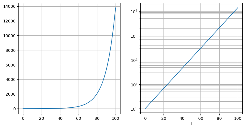
Show code cell source Hide code cell source

import numpy as np
import matplotlib.pyplot as plt

y0, mu = 1., 0.10
tv = np.arange(101)
yv = y0*(1+mu)**tv

fig, ax = plt.subplots(1,2, figsize=(10,5))
ax[0].plot(    tv, yv); ax[0].set_xlabel('t'), ax[0].grid()
ax[1].semilogy(tv, yv); ax[1].set_xlabel('t'), ax[1].grid(which="both")

(Text(0.5, 0, 't'), None)

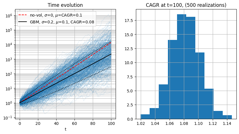
10.6.1.1. Volatility Drag

Under the assumption of normal distribution of 1-period return, the price of an asset with constant expected return \(\mu\) and variance of returns \(\sigma\) can be modelled as a geometric Brownian motion, whose compound 1-period (usually annual, and thus the acronym CAGR, compund annual growth rate) growth rate has expected value

\[CAGR = \mu - \frac{\sigma^2}{2} \ .\]

Show code cell source Hide code cell source

import numpy as np
import matplotlib.pyplot as plt

y0, mu, sig = 1., 0.10, 0.2
mu_gbm = mu - .5 * sig**2
sig_gbm = sig
nt = 101

tv = np.arange(nt)

#> Realizations
nreal = 500
#> Random number generator of the increment
rng = np.random.default_rng().normal
rng_params = {'loc': mu, 'scale': sig, 'size': nt}

yreal = np.array([ y0*np.cumprod(1 + rng(**rng_params)) for ireal in np.arange(nreal) ]).T

y_no_vol = y0*(1+mu)**tv
y_gbm_exp = y0*(1+mu_gbm)**tv

fig, ax = plt.subplots(1,2, figsize=(10,5))
ax[0].semilogy(tv, yreal, lw=.1, color=plt.cm.tab10.colors[0])
# ax[0].plot(tv, yv); ax[0].set_xlabel('t'), ax[0].grid()
ax[0].semilogy(tv, y_no_vol ,'--', color='red', label=f'no-vol, $\sigma$=0, $\mu$=CAGR={mu}')
ax[0].semilogy(tv, y_gbm_exp, '-', color='black', label=f'GBM, $\sigma$={sig}, $\mu$={mu}, CAGR={mu_gbm}')
ax[0].semilogy(tv, y_gbm_exp*np.exp(-sig*np.sqrt(tv)),':', color='black')
ax[0].semilogy(tv, y_gbm_exp*np.exp( sig*np.sqrt(tv)),':', color='black')
ax[0].set_xlabel('t'), ax[0].grid(which="both"), ax[0].legend()
ax[0].set_title('Time evolution')
ax[1].hist((yreal[-1,:])**(1/nt), density=True)
ax[1].set_title(f'CAGR at t={tv[-1]}, ({nreal} realizations)')
ax[1].grid()

todo

• “Time and risk?” Listen to The Logic of Risk

10.7. Disciplined Investing

10.7.1. Rebalancing

Colab Notebook, rebalancing.ipynb

10.7.1.1. Rebalancing premium

---

1

Even the most safe assets could undergo some (really) rare, but usually (really) catastrophic events. Just as an example, it’s hard to imagine what could happen even to bonds issued by the most (perceived and priced) safe government or institution, in case of its participation in a war.