3.9.2. Power-law distributions

Power-law distributions are an extreme case of heavy-tailed distributions. As an example, the right tail of a power-law distribution decays as \(x^\alpha\), with \(\alpha < 0\), for \(x \rightarrow +\infty\).

todo Examples of systems with power-law distributions, universality and absence of scales

• …

• Inertial scales in turbulence (Kolomogorov)

• …

3.9.2.1. Example: three different coin-flip games

Head or Tail with a fair coin, with different returns and termination events:

1. \(100\) tosses of a coin, every \(H\) gives you \(1\$\). The probability distribution of the total return is the binomial distribution. With the definition of a Bernoulli random variable \(X_i = 1\) for \(H\), \(X_i = 0\) for \(T\) with even probability, the amount at the end of the game, after \(n=100\) tosses, reads

   \[w_{end} = \sum_{i=1}^n X_i \cdot 1\$ \ .\]

2. \(100\) tosses, an \(H\) gives you \(g=+10\%\) gain a \(T\) produces a \(\ell=-10\%\) loss of the amount you have. At any coin toss, you bet eveything you have. This problem looks like compounding in investing1. Starting with \(r_0 = 1\$\), the amount at the end of the game, after \(n\) tosses, reads

   \[w_{end} = w_0 \prod_{i=1}^n ( 1 + g )^{X_i} ( 1 + \ell )^{1 - X_i} \ . \]

3. \(100\) tosses, getting \(H\) you win \(g=+10\%\), getting \(T\) you win nothing and the game stops: first \(T\) is the termination event; starting with \(1\$\), after the \(n^{th}\) \(H\) in a row, you have \(1\$ \cdot 1.1^n\). The amount at the end of the game reads

   \[\begin{split}w_{end} = \begin{cases} w_0 \cdot (1+g)^{n_H} & \text{with probability $2^{-1-n_H}$ for $n_H < n_{tosses}$} \\ w_0 \cdot (1+g)^{n_H} & \text{with probability $2^{-n_{tosses}}$ for $n_H = n_{tosses}$} \end{cases}\end{split}\]

   being \(n_H\) the number of \(H\) in a row. If \(n_H\) is constrained to be \(\le n_{tosses} = 100\), the probability of getting exactly \(99\) or \(100\) \(H\) in a row is the same; if \(n_H\) is not constrained, \(w_{end} = w_0 \cdot (1+g)^{n_H}\), for all \(n_H \ge 0\), with \(p(n_H) = \frac{1}{2^{1+n_H}}\).

Show code cell source Hide code cell source

%reset -f
import numpy as np
import scipy as sp
import matplotlib.pyplot as plt

n_tosses = 30
p_head = .5

#> 1.Binomial distribution
lb, ub = sp.stats.binom.support(n_tosses, p_head)
xv_binom = np.arange(lb, ub+1)
p_binom = sp.stats.binom.pmf(xv_binom, n_tosses, p_head)
print(lb, ub)

#> 2. Compounding
gain, loss = .15, -.15
nv = np.arange(0, n_tosses+1)
xv_comp = np.array([ (1.+gain)**n * (1.+loss)**(n_tosses-n) for n in nv])
# p_binom = sp.stats.binom.pmf(xv_binom, n_tosses, p_head)


#> 3. Power-law distibution
xv_power = (1+gain)**nv
p_power = 2.**(-1.-nv)

fig, ax = plt.subplots(1,4, figsize=(15, 3))
ax[0].plot(xv_binom, p_binom, 'o')
ax[0].plot(xv_comp , p_binom, 'o')
ax[0].plot(xv_power, p_power, 'o')

ax[1].semilogx(xv_binom, p_binom, 'o')
ax[1].semilogx(xv_comp , p_binom, 'o')
ax[1].semilogx(xv_power, p_power, 'o')

ax[2].semilogy(xv_binom, p_binom, 'o')
ax[2].semilogy(xv_comp , p_binom, 'o')
ax[2].semilogy(xv_power, p_power, 'o')

ax[3].loglog(xv_binom, p_binom, 'o', label='Binomial')
ax[3].loglog(xv_comp , p_binom, 'o', label='Compounding')
ax[3].loglog(xv_power, p_power, 'o', label='Power-law')
ax[3].legend()

for i in np.arange(4): ax[i].grid()

0 30

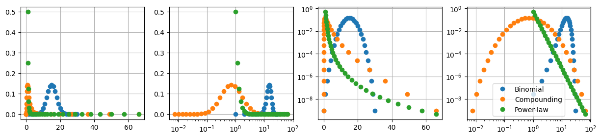
• Binomial distribution becomes approximately normal as \(n\) increases,

  \[p_1(x) \sim \mathscr{N}(\mu_n, \sigma_n) \sim \text{exp} \left[ -\frac{(x-\mu_n)^2}{2 \sigma^2_n} \right]\]

• Compounding produces a distribution that becomes approximately log-normal as \(n\) increases…

• Power-law has probability \(p_3(n)\) and outcome \(x_3(n)\)

  \[p_3(n) = 2^{-1-n} \quad , \quad x_3(n) = 2^n \ ,\]

  and thus \(p_3(x) = \frac{1}{2} x^{-1} \ .\) Taking the logarithm of this expression, a 1-degree polynomial relation between logarithms of \(p\) and \(x\) is obtained, \(\ln p_3 = - \ln 2 - \ln x\).

3.9.2.2. Integrability of tails, existence of moments

Power-law pdf and existence of moments.

A power-law density \(p(x) \propto x^{\alpha}\) defined on an unbounded domain is normalizable only for \(\alpha < -1\). For \(\alpha \ge -1\), normalization requires the introduction of an upper cutoff.

On unbounded domains, the first \(n\) moments exist if \(\alpha > -n\).

Let the tail of the distribution follow a power law \(p(x) \sim x^\alpha\) for \(x > x_0\). On finite domains, no problem exists. On infinite domains, in order for \(p(x)\) to represent a probability density function, \(\alpha < -1\), as

\[\begin{split}\int_{x = x_0}^{+\infty} p(x) \, dx = \int_{x = x_0}^{+\infty} x^{\alpha} \, dx = \left.\frac{1}{1+\alpha} x^{1+\alpha} \right|_{x_0}^{+\infty} = \begin{cases} -\frac{1}{1+\alpha} x_0 \ \text{ finite } & , \ \alpha < -1 \\ \infty & , \ \alpha \ge -1 \end{cases} \end{split}\]

Even if the function \(p(x)\) is a pdf, \(\alpha < -1\), moments may diverge.

Expected value.

\[\mu = \int_{\Omega} x \, p(x) \, dx\]

if \(\Omega\) has no upper limit, the integral converges only if

\[\int_{x_0}^{+\infty} x \, p(x) \, dx \sim \int_{x_0}^{+\infty} x \cdot x^{\alpha} \, dx = \int_{x_0}^{+\infty} x^{\alpha+1} \, dx \ ,\]

converges, i.e. for \(\alpha < -2\)

Variance. Analogously, the distribution has finite variance if \(\alpha < -3\).

3.9.2.3. Failure of CLT

Using transformation of probability functions to sample a r.v. with power-law distribution \(p(x) = c x^{-\alpha}\), \(x \in [x_0, +\infty)\), starting from sampling of a r.v. with uniform distribution \(u(x)=1\), \(x \in [0,1]\).

Normalization. For \(\alpha > 1\),

\[1 = \int_{t=x_0}^{+\infty} p(x) \, dx = \int_{t=x_0}^{+\infty} c x^{-\alpha} \, dx = \frac{c}{1-\alpha} \left.\left[ x^{1-\alpha} \right]\right|_{x_0}^{+\infty} = \frac{c}{\alpha - 1} x_0^{-(\alpha-1)} \ , \]

and thus \(c = (\alpha - 1 ) x_0^{\alpha-1}\), and the probability density function reads

\[p(x) = (\alpha - 1)x_0^{\alpha-1} x^{-\alpha} \ , \quad x \ge x_0 \ .\]

Expected value.

\[\begin{split}\begin{aligned} \mu & = \int_{x=x_0}^{+\infty} x \, p(x) \, dx = \\ & = \int_{x=x_0}^{+\infty} (\alpha-1) x_0^{\alpha-1} x \cdot x^{-\alpha} \, dx = \\ & = \left. (\alpha-1) x_0^{\alpha-1} \frac{1}{-\alpha+2} x^{-\alpha+2} \right|_{x_0}^{+\infty} \end{aligned}\end{split}\]

converges for \(\alpha > 2\),

\[\mu = \frac{\alpha-1}{\alpha-2} x_0 \ .\]

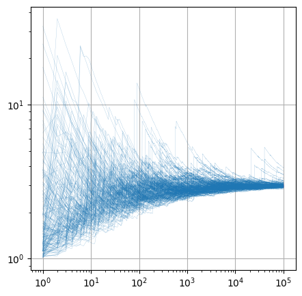
As an example, with \(\alpha = 1.5\) the expected value is not defined; with \(\alpha = 2.5\), \(\mu_{\alpha=2.5} = \frac{1.5}{0.5} x_0 = 3 x_0\).

Cumulative probability function.

\[P(x) = \int_{t=x_0}^{x} p(t) \, dt = \int_{t=x_0}^{x} c t^{-\alpha} \, dt = (\alpha - 1) x_0^{\alpha-1} \left. \frac{t^{1-\alpha}}{1-\alpha} \right|_{x_0}^{x} = 1 - \left( \frac{x_0}{x} \right)^{\alpha-1}\]

As sampling from a uniform distribution requires the equality of the cumulative probability densities, and \(U(x) = x\), todo quite bad notation it follows

\[P(X) = U \sim \text{Uniform}(0,1)\]

and thus

\[U = 1 - \left( \frac{x_0}{X} \right)^{\alpha-1}\]

or

\[X = x_0 \, \left( 1 - U \right)^{-\frac{1}{\alpha - 1}}\]

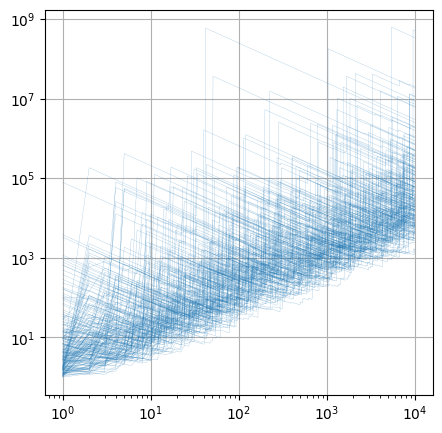
3.9.2.3.1. Power-law with \(\alpha = 1.5\)

Show code cell source Hide code cell source

%reset -f
import numpy as np

#> Power-law
x0 = 1.
alpha = 1.5

#> N.samples
n_samples = int(1e+4)
n_reals = 200

#> Uniform random number generator
rng = np.random.default_rng()
rng_uniform_fun =  lambda n: rng.uniform(.0,1., n)

um, xm = [], []

for i_real in np.arange(n_reals):
    #> Samples from the r.v. with the uniform distribution
    u = rng_uniform_fun(n_samples)

    #> Samples from the r.v. with power-law distribution
    x = x0 * ( 1. - u )**(-1./(alpha-1.))

    um += [ u ]
    xm += [ x ]

xm = np.array(xm)

Show code cell source Hide code cell source

# print(xm)
# print(np.shape(np.cumsum(xm, axis=0)))

Show code cell source Hide code cell source

import matplotlib.pyplot as plt

fig, ax = plt.subplots(1,1, figsize=(5,5))
# ax.plot( np.cumsum(xm.T, axis=0) / np.arange(1,n_samples+1)[:, np.newaxis], color=plt.cm.tab10.colors[0], lw=.5 )
ax.loglog( np.arange(1, n_samples+1),
           np.cumsum(xm.T, axis=0) / np.arange(1,n_samples+1)[:, np.newaxis], 
           color=plt.cm.tab10.colors[0], 
           alpha=.5,
           lw=.2 )
ax.grid()

plt.show()

3.9.2.3.2. Power-law with \(\alpha = 2.5\)

Show code cell source Hide code cell source

%reset -f
import numpy as np

#> Power-law
x0 = 1.
alpha = 2.5

#> N.samples
n_samples = int(1e+5)
n_reals = 200

#> Uniform random number generator
rng = np.random.default_rng()
rng_uniform_fun =  lambda n: rng.uniform(.0,1., n)

um, xm = [], []

for i_real in np.arange(n_reals):
    #> Samples from the r.v. with the uniform distribution
    u = rng_uniform_fun(n_samples)

    #> Samples from the r.v. with power-law distribution
    x = x0 * ( 1. - u )**(-1./(alpha-1.))

    um += [ u ]
    xm += [ x ]

xm = np.array(xm)

Show code cell source Hide code cell source

import matplotlib.pyplot as plt

fig, ax = plt.subplots(1,1, figsize=(5,5))
# ax.plot( np.cumsum(xm.T, axis=0) / np.arange(1,n_samples+1)[:, np.newaxis], color=plt.cm.tab10.colors[0], lw=.5 )
ax.loglog( np.arange(1, n_samples+1),
           np.cumsum(xm.T, axis=0) / np.arange(1,n_samples+1)[:, np.newaxis], 
           color=plt.cm.tab10.colors[0], 
           alpha=.5,
           lw=.2 )
ax.grid()

plt.show()

todo Plot

• max \(M_n\) vs. sum \(S_n\), as the ratio \(\frac{M_n}{S_n}\) as max dominates sum for heavy-tailed distributions

• quantile trajectories

todo Let’s check the following results, with Law of Large Numbers (LLN) and Central Limit Theorem (CLT)

(\alpha)	Mean	Variance	Sample mean behavior
\(\alpha>3\)	Finite	Finite	Classical LLN & CLT (Gaussian)
\(2<\alpha \le 3\)	Finite	Infinite	LLN holds, but CLT replaced by stable law (non-Gaussian fluctuations)
\(\alpha \le 2\)	Infinite	Infinite	LLN fails, sample mean diverges; dominated by extreme events

---

1

The probability distribution of the total return can be easily derived withminor modifications from the derivation of the Kelly criterion, Example 10.3, an optimality criterion for this game, if you can choose the fraction of the amount you have for betting, given the gain and loss.