Show the code
#> Import libraries
%reset -f
import numpy as np
import scipy as sp

import matplotlib.pyplot as plt

import plotly.express as px
import plotly.io as pio
import pandas as pd

pio.renderers.default = "notebook"Humans are wired to find patterns in randomness. If a coin lands on Heads five times in a row, our intuition insists something is up. But how do we separate a genuine structural change from mere background noise?
An answer can be provided using Hypothesis Testing. This statistical framework strips away human subjectivity - or at least define it before performing experiments and quantify its consequences - and quantifies our beliefs. By setting an initial assumption—the Null Hypothesis (\(H_0\)), such as a perfectly fair coin—we can mathematically calculate whether our observations are a random fluke or a definitive anomaly.
This post contains three sections:
Coin tosses have no memory: \(50.000\) tosses of a fair coin is modeled as independent random variables, and sample data are discussed to show that random independent events have no memory, debunking the myth of the “hot hand.”
10 heads in a row: in the first section a definition of fair coin is used, and trusted. But how can be infer/know that a coin is fair from a sequence of its outcomes? This section aims at using hypotesis testing to provide an answer
The Bayesian alternative
#> Import libraries
%reset -f
import numpy as np
import scipy as sp
import matplotlib.pyplot as plt
import plotly.express as px
import plotly.io as pio
import pandas as pd
pio.renderers.default = "notebook"We know that a coin is fair, so that its outcome has the probability of 50% to be head (\(H\)) and 50% to be tail (\(T\)). Mathematically, the outcome of a coin toss can be modelled as Bernoulli random variable with \(p_{\text{H}} = 0.5\) and \(p_{\text{T}} = 1 - p_{\text{H}} = 0.5\).
\[p(X) = \left\{ \begin{aligned} & p_{\text{H}} & , \quad \text{X} = \text{H} \\ & 1 - p_{\text{H}} & , \quad \text{X} = \text{T} \\ \end{aligned} \right. \tag{1}\]
One may ask how does one know that the coin is fair?, and an answer to this question is provided in the next section.
If coin tosses can be treated as independent events1, the outcomes of a toss or a sequence of tosses do not influence the outcome of the following.
Next experiment tries to show the validity of this assumption. Coin tosses are modelled as i.i.d. random variables with a uniform Bernoulli random variable. The results of a coin toss is modelled as a sample from this distribution. Here, \(N_{tosses} = 50.000\) tosses are performed. Data is collected, and the conditional probability of getting \(H\) or \(T\) after a streak of \(n\) Heads in a row is sampled. The empirical probability of getting \(H\) is computed, and used to assess the validity of the assumption through hypotesys testing: for more about inferential hypotesis testing, see the link or the paragraph below. Different values of \(n\) are investigated, to show that:
# 1. Set seed for reproducibility and simulate 50,000 coin tosses
# 0 = Tails (T), 1 = Heads (H)
# np.random.seed(42)
num_tosses = 50_000
tosses = np.random.randint(0, 2, size=num_tosses)

# 2. Analyze the outcomes following a streak of 'n' consecutive Heads
max_n = 8
results = []

for n in range(1, max_n + 1):
    streak_count = 0
    next_is_head = 0
    next_is_tail = 0

    # Slide a window across the array to find streaks
    # We stop at len(tosses) - 1 because we need to look at the subsequent toss
    for i in range(num_tosses - n):
        # Check if the previous 'n' tosses were all Heads (1)
        if np.all(tosses[i:i+n] == 1):
            streak_count += 1
            # Look at the immediate next toss (index i + n)
            if tosses[i+n] == 1:
                next_is_head += 1
            else:
                next_is_tail += 1

    # Calculate empirical probabilities
    p_head = (next_is_head / streak_count) * 100 if streak_count > 0 else 0
    p_tail = (next_is_tail / streak_count) * 100 if streak_count > 0 else 0

    # Calculate the 95% Confidence Interval margin of error for a fair coin (p=0.5)
    # SE = sqrt(p*(1-p)/N), Margin of Error = 1.96 * SE
    if streak_count > 0:
        margin_of_error = 1.96 * np.sqrt((0.5 * 0.5) / streak_count) * 100
    else:
        margin_of_error = 0.0

    results.append({
        "Streak Length, n": n,
        "Total Matches": streak_count,
        "Next is H": next_is_head,
        # "Next is T": next_is_tail,
        "Empirical P(H)": f"{p_head:.2f}%",
        "95% CI Limits": f"{50 - margin_of_error:.2f}% - {50 + margin_of_error:.2f}%",
        "95% CI Half-Width": f"{margin_of_error:.2f}%",
    })

# Display the results neatly
df = pd.DataFrame(results)
display(df)
# print(df.to_string(index=False))| Streak Length, n | Total Matches | Next is H | Empirical P(H) | 95% CI Limits | 95% CI Half-Width | |
|---|---|---|---|---|---|---|
| 0 | 1 | 25097 | 12607 | 50.23% | 49.38% - 50.62% | 0.62% |
| 1 | 2 | 12607 | 6338 | 50.27% | 49.13% - 50.87% | 0.87% |
| 2 | 3 | 6338 | 3234 | 51.03% | 48.77% - 51.23% | 1.23% |
| 3 | 4 | 3234 | 1669 | 51.61% | 48.28% - 51.72% | 1.72% |
| 4 | 5 | 1669 | 875 | 52.43% | 47.60% - 52.40% | 2.40% |
| 5 | 6 | 875 | 471 | 53.83% | 46.69% - 53.31% | 3.31% |
| 6 | 7 | 471 | 253 | 53.72% | 45.48% - 54.52% | 4.52% |
| 7 | 8 | 253 | 150 | 59.29% | 43.84% - 56.16% | 6.16% |
The empirical probability of getting \(H\) after a streak of \(n\) \(H\) is approximatley \(50%\). This is a qualitatively information. But how close to \(50\%\) is close enough? I could think \(49.5\%\) is not enough to prove the assumption, you could think \(55.5\%\) is fair enough.
We can’t cut subjectivity as a whole, but hypthesis testing provides a framework to work with. Level of significance \(\alpha\) - representing the subjectivity - represents the the probability of rejecting a true null hypothesis (Type I erro/false positive). * A statement is made, the null hypotesis \(H_0\) * A test statistics of data under \(H_0\) is chosen, so that the probability \(p(x|H_0)\) is known * Data is sampled, and the estimate \(\hat{x}\) of the test statistics is evaluated with the samples * The properties of the statistical test (one- or two-tail test, reference value,…) are chosen * Acceptance and rejection regions - depending on \(\alpha\) - are evaluated * Null hypotesis is rejected if \(\hat{x}\) belongs to the rejection region
Here the level of acceptance - the probability of not-rejecting a false claim - \(\alpha = 5\%\) is chosen; the test statistics \(x\) is chosen as the average value of the coin tosses after the desired streaks, or the ratio of the number of heads over the number of tosses after the desired streaks; the ratio of head outcomes after the desired streaks - i.e. the estimated value \(\hat{x}\) - is counted; this value is checked against the rejection region.
Relying on the central limit theorem, here the acceptance region is defined for a Gaussian distribution - well approximating the binomial distribution of sequences of independent Bernoulli events. For a given value of \(\alpha\), the half-width of the \(95\%\) intervals scales with the number of samples, here the Total Matches, as
\[1.96 \frac{\sigma}{\sqrt{N_{matches}}} \ ,\]
and thus ranging from \(0.62\%\) to \(7.32\%\) as the streak length goes from \(1\) to \(8\) and the number occurrences of \(n\)-length streaks goes from \(25.000\) to \(180\).
The table shows that the actual ratio of \(H\) as an outcome after \(n\)-\(H\) streaks belongs to the \(95\%\) confidence interval, i.e. the acceptance region.
The problem is a bit different from the one of the first section. You walk up to a table and know nothing about the croupier and the dice. You start watching the table and the first 10 tosses you observe are all heads. Is it reasonable to think you’re observing a rare event for a fair coin, or should you start blaming the coin?
Probability \(p_N(n)\) of \(n\) Head outcomes in \(N\) tosses of a fair dice. With a fair dice, the probability of observe \(n\) Heads in \(N\) tosses is represented by the binomial distribution
\[p_N(n) = \left( \begin{matrix} N \\ n \end{matrix} \right) p_{\text{H}}^n ( 1 - p_{\text{H}} )^{N-n} \tag{2}\]
#> Possible outcomes of the n. of observed Heads in n_flips
n_flips = 10
heads_v = np.arange(n_flips+1)
xv = heads_v # / n_flips     # If required, normalization

#> Discrete probability density for a fair coin
p_head_fair = .5
x_H0_fv = sp.stats.binom.pmf(heads_v, n_flips, p_head_fair)#> Plotly image
#> Dataframe collecting n.of head outcomes and their probability
df = pd.DataFrame({
'Number of Heads (n)': heads_v,
'Probability': x_H0_fv
})
#> Plotly figure
fig = px.bar(df, x='Number of Heads (n)', y='Probability',
title='Probability of Observing n Heads in 10 Coin Tosses',
labels={'Number of Heads (n)': 'Number of Heads (n)', 'Probability': 'Probability'},
text_auto='.4f')
fig.update_layout(
xaxis=dict(tickmode='linear', tick0=0, dtick=1),
title_x=0.5
)
fig.show()The probability of observing \(N\) heads in \(N\) tosses with a fair coin goes as
\[P_N(N) = \frac{1}{2^N} \ ,\]
as it’s the joint probability of \(N\) independent events with individual probability \(p_{\text{H,fair}} = \frac{1}{2}\). So, while there \(50\%\) - i.e. \(1/2\) - probability of observing \(H\) in a toss, \(25\%\) - i.e. \(1/4\) - of observing \(HH\) in 2 tosses, there’s less than \(1/1000\) probability of observing \(10 \, \text{H}\) in a row in \(10\) tosses with a fair coin.
| \(N\) | \(p_N(N)\) |
|---|---|
| \(1\) | \(0.5\) |
| \(2\) | \(0.25\) |
| \(3\) | \(0.125\) |
| \(4\) | \(6.25 \cdot 10^{-2}\) |
| \(5\) | \(3.125 \cdot 10^{-2}\) |
| \(6\) | \(1.56 \cdot 10^{-2}\) |
| \(7\) | \(7.81 \cdot 10^{-3}\) |
| \(8\) | \(3.91 \cdot 10^{-3}\) |
| \(9\) | \(1.95 \cdot 10^{-3}\) |
| \(10\) | \(9.77 \cdot 10^{-4}\) |
Inferring if a coin is fair. With Fisher method for hypothesis testing, * a null assumption \(\text{H}_0\) is formulated, and believed true until it’s not believed true anymore - i.e. it’s falsified. This null assumption is usually formulated with a test statistics \(x\) whose conditioned probability under the null assumption \(p(x | \text{H}_0)\) is known * the method (1- or 2-tail test) and the level of significance \(\alpha\) of the test are chooen. These choises determin the rejection region \(A_r(\alpha)\) and the acceptance region \(A_a(\alpha)\) of the test statistics * samples are collected and the test statistics \(\hat{x}\) is evaluated (estimated, since we’re trying to evaluate a random variable through samples - see as an example Estimators; sample mean and variance) with these samples * comparison of the estimate \(\hat{x}\) of the test statistics with the rejection region \[\begin{aligned} \hat{x} \in A_r(\alpha) \quad \rightarrow \quad \text{the test falsifies H}_0 \end{aligned}\]
As the level of significance \(\alpha\) increases, the rejection region becomes smaller and smaller, so the need for evidence increases.
Here the coin toss is modelled as a Bernoulli stochastic variable. Different coins with “different levels of fairiness” are uniquely defined by the probability \(p_{\text{H}}\) of the head event. Here different coins are evaluated with
\[p_{\text{H}} \in \left\{ 0.5, 0.45, 0.4, 0.3, 0.2, 0.1 \right\} \ .\]
Routines for running the experiments and evaluating the acceptance regions are defined.
#> Random process of interest, unknown execpt for the sample.
p_head_default = .5
p_tail_default = 1. - p_head_default

# Coin flip as a Bernoulli probability with outcomes: a = [0, 1] with prob p = [p_head, p_tail]
flip_rng_default = np.random.default_rng(42).choice
flip_params_default = { 'a': [0,1], 'p': [p_head_default, p_tail_default], 'size': 1 }   # default params

def run_experiment(rng=flip_rng_default, rng_params=flip_params_default):
return rng(**rng_params)def px_H0(p, p_params,):
return p(**p_params)#> Acceptance and rejection regions, for discrete pdf
# Starting from the value of the test statistics x_max = max(x_H0_fv), expand
def find_acceptance_region(p, alpha, test_type='value'):
"""
Find acceptance region for a discrete pdf, supposed to be unimodal
for a given value of significance level
test_type is not used so far...
"""
x_max = np.argmax(p)
nx = len(p)
threshold = 1. - alpha
# Initialization
p_acc, xl, xr = p[x_max], x_max, x_max
# if ( test_type == 'value' ):
while ( p_acc < threshold ):
if ( p[xl-1] >= p[xr+1] ):
xl -= 1; p_acc += p[xl]
else:
xr += 1; p_acc += p[xr]
# else:
return xl, xr
def find_acceptance_regions(p, alpha_v, test_type='value'):
"""
Find acceptance region for a discrete pdf, supposed to be unimodal
for a set of values of significance levels, type(alpha_v) = numpy.array
test_type is not used so far...
"""
#> Dimensions
ix_max = np.argmax(p)
nx, nal = len(p), len(alpha_v)
ixlv, ixrv = np.zeros(nal), np.zeros(nal)
#> Sorting
alpha_v = np.sort(alpha_v)[::-1]
threshold_v = 1. - alpha_v
# Initialization
p_acc, ixl, ixr = p[ix_max], ix_max, ix_max
#> Loop over all the thresholds
for ial in np.arange(nal):
while ( p_acc < threshold_v[ial] ):
if ( p[ixl-1] > p[ixr+1] ):
ixl -= 1; p_acc += p[ixl]
else:
ixr += 1; p_acc += p[ixr]
ixlv[ial], ixrv[ial] = ixl, ixr
return ixlv, ixrv
#> Test
# n_flips = 160
# x_H0_fv = sp.stats.binom.pmf(np.arange(n_flips+1), n_flips, .5) # p_fair_coin .5
# xlv, xrv = find_acceptance_regions(x_H0_fv, alpha_v,)
# print(xlv, xrv)Different levels of significance are defined, to show its influence on the acceptance region and on the inference test later.
#> Test characteristics: symmetric
# test_type = 'value'  # 'symmetric', 'right', 'left', 'value'

#> Significance level, alpha = .05 ("default")
alpha = .05
alpha_v = np.array([ .3, .05, .003 ])#> Run experiments, with incremental number of samples
n_flips_1 = 20
n_flips_max = 10_000
n_flips = 0
H0_true = True
ov_fair, ov_rigg = [], []
ov_rig4, ov_rig3, ov_rig2, ov_rig1 = [], [], [], []
xlv, xrv, xsv_fair, xsv_rigg, n_flipsv = [], [], [], [], []
xsv_rig4, xsv_rig3, xsv_rig2, xsv_rig1 = [], [], [], []
flip_rng = np.random.default_rng().choice
flip_params_fair = { 'a': [0,1], 'p': [.5 , .5 ], 'size': n_flips_1 } # default params
flip_params_rigg = { 'a': [0,1], 'p': [.48, .52], 'size': n_flips_1 } # default params
# flip_params_rigg = { 'a': [0,1], 'p': [.45, .55], 'size': n_flips_1 } # default params
flip_params_rig4 = { 'a': [0,1], 'p': [.4 , .6 ], 'size': n_flips_1 } # default params
flip_params_rig3 = { 'a': [0,1], 'p': [.3 , .7 ], 'size': n_flips_1 } # default params
flip_params_rig2 = { 'a': [0,1], 'p': [.2 , .8 ], 'size': n_flips_1 } # default params
flip_params_rig1 = { 'a': [0,1], 'p': [.1 , .9 ], 'size': n_flips_1 } # default params
while ( n_flips < n_flips_max and H0_true ):
#> Run a new experiment and collect new n_flips_1 samples
n_flips += n_flips_1
ov_fair_1 = run_experiment(rng=flip_rng, rng_params=flip_params_fair)
ov_rigg_1 = run_experiment(rng=flip_rng, rng_params=flip_params_rigg)
ov_rig4_1 = run_experiment(rng=flip_rng, rng_params=flip_params_rig4)
ov_rig3_1 = run_experiment(rng=flip_rng, rng_params=flip_params_rig3)
ov_rig2_1 = run_experiment(rng=flip_rng, rng_params=flip_params_rig2)
ov_rig1_1 = run_experiment(rng=flip_rng, rng_params=flip_params_rig1)
ov_fair += list(ov_fair_1)
ov_rigg += list(ov_rigg_1)
ov_rig4 += list(ov_rig4_1)
ov_rig3 += list(ov_rig3_1)
ov_rig2 += list(ov_rig2_1)
ov_rig1 += list(ov_rig1_1)
#> Find distribution function
x_H0_fv = px_H0(sp.stats.binom.pmf, {'k': np.arange(0,n_flips+1), 'n': n_flips, 'p': .5}) # H0: fair coin
#> Evaluate acceptance region
ixl, ixr = find_acceptance_regions(x_H0_fv, alpha_v,)
# print(n_flips, ixl, ixr)
#> Evaluate test statistics on the sample
ixs_fair = np.sum(ov_fair)
ixs_rigg = np.sum(ov_rigg)
ixs_rig4 = np.sum(ov_rig4)
ixs_rig3 = np.sum(ov_rig3)
ixs_rig2 = np.sum(ov_rig2)
ixs_rig1 = np.sum(ov_rig1)
#> Check if H0 is not false. If commented, let the while run until n_flips = n_flips_max
# if ( ixl[-1] > ix_s or ixr[-1] < ix_s ):
# H0_true = False
#> Store quantities for plots
n_flipsv += [ n_flips ]
xlv += [ ixl/n_flips ]
xrv += [ ixr/n_flips ]
xsv_fair += [ ixs_fair/n_flips ]
xsv_rigg += [ ixs_rigg/n_flips ]
xsv_rig4 += [ ixs_rig4/n_flips ]
xsv_rig3 += [ ixs_rig3/n_flips ]
xsv_rig2 += [ ixs_rig2/n_flips ]
xsv_rig1 += [ ixs_rig1/n_flips ]
Results are shown. The outcome of the coin toss is converted to a \(\{ 0, 1 \}\) coding, as \(H \rightarrow 0\), \(T \rightarrow 1\). The test statistics
A scaled version is shown to make the acceptance regions approximately independent from the number \(n\). As the events are independent and identically distributed with expected value \(\overline{x}\) and finite variance \(\sigma^2\), the average of the outcomes
\[\hat{x} = \frac{1}{n} \sum_{j=1}^{n} x_n \ ,\]
tends to a random variable with Gaussian distribution \(\mathscr{N}\left( \mu, \frac{\sigma^2}{n} \right)\), for the central limit theorem. This observation seamlessly induces a useful scaling of the test variable
\[\frac{\hat{x} - \mu}{\sigma/\sqrt{n}} \sim \mathscr{N}\left( 0, 1 \right) \ .\]
#> Convert list to numpy arrays, to perform some algebra below
n_flipsv = np.array(n_flipsv)
xlv = np.array(xlv)
xrv = np.array(xrv)
xsv_fair = np.array(xsv_fair)
xsv_rigg = np.array(xsv_rigg)
xsv_rig4 = np.array(xsv_rig4)
xsv_rig3 = np.array(xsv_rig3)
xsv_rig2 = np.array(xsv_rig2)
xsv_rig1 = np.array(xsv_rig1)

#>
plt.figure(figsize=(10,5))
plt.subplot(1,2,1)
for ial in np.arange(len(alpha_v)):
    # plt.plot(n_flipsv, xlv[:,ial], color=plt.cm.tab10(ial))
    # plt.plot(n_flipsv, xrv[:,ial], color=plt.cm.tab10(ial))
    plt.fill_between(n_flipsv,
                     xlv[:,ial],
                     xrv[:,ial], color=(0,0,0,.1))
plt.plot(n_flipsv, xsv_fair, color=plt.cm.tab10(0), label='fair')
plt.plot(n_flipsv, xsv_rigg, color=plt.cm.tab10(1), label='rigged, .48')
plt.plot(n_flipsv, xsv_rig4, color=plt.cm.tab10(2), label='rigged, .4')
plt.plot(n_flipsv, xsv_rig3, color=plt.cm.tab10(3), label='rigged, .3')
plt.plot(n_flipsv, xsv_rig2, color=plt.cm.tab10(4), label='rigged, .2')
plt.plot(n_flipsv, xsv_rig1, color=plt.cm.tab10(5), label='rigged, .1')

plt.plot(n_flipsv, .5 *np.ones(np.shape(xsv_fair)), '--', color=plt.cm.tab10(0))
plt.plot(n_flipsv, .52*np.ones(np.shape(xsv_fair)), '--', color=plt.cm.tab10(1))
plt.plot(n_flipsv, .6 *np.ones(np.shape(xsv_fair)), '--', color=plt.cm.tab10(2))
plt.plot(n_flipsv, .7 *np.ones(np.shape(xsv_fair)), '--', color=plt.cm.tab10(3))
plt.plot(n_flipsv, .8 *np.ones(np.shape(xsv_fair)), '--', color=plt.cm.tab10(4))
plt.plot(n_flipsv, .9 *np.ones(np.shape(xsv_fair)), '--', color=plt.cm.tab10(5))

plt.xlim(0, n_flips)
#plt.ylim(-5, 5)
plt.title("Avg outcome, $\hat{x}_s(n_s)$")
plt.xlabel('$n_s$')
plt.legend()
plt.grid()

#> For scaling results
bernoulli_avg, bernoulli_var = .5, .25

plt.subplot(1,2,2)
for ial in np.arange(len(alpha_v)):
    # plt.plot(n_flipsv, xlv[:,ial], color=plt.cm.tab10(ial))
    # plt.plot(n_flipsv, xrv[:,ial], color=plt.cm.tab10(ial))
    plt.fill_between(n_flipsv,
                     (xlv[:,ial]-bernoulli_avg) * n_flipsv**.5/bernoulli_var**.5,
                     (xrv[:,ial]-bernoulli_avg) * n_flipsv**.5/bernoulli_var**.5, color=(0,0,0,.1))
plt.plot(n_flipsv, (xsv_fair-bernoulli_avg) * n_flipsv**.5/bernoulli_var**.5, color=plt.cm.tab10(0), label='fair')
plt.plot(n_flipsv, (xsv_rigg-bernoulli_avg) * n_flipsv**.5/bernoulli_var**.5, color=plt.cm.tab10(1), label='rigged, .48')
plt.plot(n_flipsv, (xsv_rig4-bernoulli_avg) * n_flipsv**.5/bernoulli_var**.5, color=plt.cm.tab10(2), label='rigged, .4')
plt.plot(n_flipsv, (xsv_rig3-bernoulli_avg) * n_flipsv**.5/bernoulli_var**.5, color=plt.cm.tab10(3), label='rigged, .3')
plt.plot(n_flipsv, (xsv_rig2-bernoulli_avg) * n_flipsv**.5/bernoulli_var**.5, color=plt.cm.tab10(4), label='rigged, .2')
plt.plot(n_flipsv, (xsv_rig1-bernoulli_avg) * n_flipsv**.5/bernoulli_var**.5, color=plt.cm.tab10(5), label='rigged, .1')
plt.grid()

plt.plot(n_flipsv, ( .5*np.ones(np.shape(xsv_fair))-bernoulli_avg) * n_flipsv**.5/bernoulli_var**.5, '--', color=plt.cm.tab10(0))
plt.plot(n_flipsv,-(.48*np.ones(np.shape(xsv_fair))-bernoulli_avg) * n_flipsv**.5/bernoulli_var**.5, '--', color=plt.cm.tab10(1))
plt.plot(n_flipsv,-( .4*np.ones(np.shape(xsv_fair))-bernoulli_avg) * n_flipsv**.5/bernoulli_var**.5, '--', color=plt.cm.tab10(2))

plt.xlim(0, n_flips)
plt.ylim(-5, 5)
plt.title("Scaled avg outcome, $\dfrac{\hat{x}_s - \overline{x}}{\sigma/\sqrt{n}}$")
plt.xlabel('$n_s$')
plt.legend()
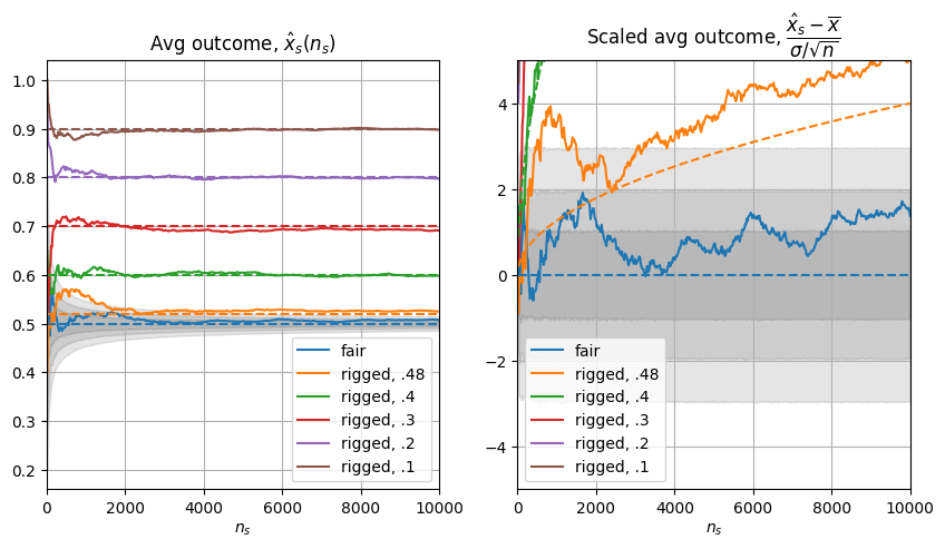
Acceptance regions for different statistical significance levels are shown in grayscale. The widest, most conservative acceptance region corresponds to \(\alpha = 0.003\) (the standard industrial \(\sim3\sigma\) control limit). The intermediate region corresponds to \(\alpha = 0.05\) (the standard scientific \(\sim2\sigma\) limit), and the narrowest, most sensitive region corresponds to \(\alpha = 0.3\) (a loose \(\sim 1\sigma\) limit).
The right plot shows that 2000 tosses may not be enough to reject the assumption of fairness for a subtly rigged coin (\(48\%\) - \(52\%\) split).
In this section, Bayesian approach is applied for testing a hypothesis. After a coin is tossed \(n\) times and the outcome is Head \(n_H\) times, the question is: with the observed data, what’s the probability of Heads in a single coin toss?
Here, the coin toss is modeled as a Bernoulli random variable with probability density Equation 1, and the value \(p_H\) of the probability of getting Head needs to be estimated, using available data.
So, here: * the model is given: the random variable is modeled with a Bernoulli random variable * the parameters of the models need to be determined: the model has only one parameter \(p_H\)
In this section, the symbol \(f\) is used for probability densities, just to avoid too many \(p\)s.
Using a coin with probability of Head outcome equal to \(p_H\), the probability of observing \(x\) Heads in \(n\) tosses is given by the expression Equation 2,
\[f(n_H, n | p_H) = \left( \begin{matrix} n \\ n_H \end{matrix} \right) p_{\text{H}}^{n_H} ( 1 - p_{\text{H}} )^{n-n_H} \ . \tag{3}\]
In order to apply Bayes’ theorem
\[f(y|x) = \frac{f(x|y) f(y)}{f(x)} \ , \tag{4}\]
to get a probability distribution for the parameters of the model \(y\), given the observed data \(x\), i.e. \(p(y|x)\), one needs:
a prior \(f(y)\), i.e. a (plausible) distribution of the parameters \(y\).
a likelihood function, i.e. the conditional probability \(f(x|y)\) of observing data \(x\), given the value \(y\) of the parameters of the model
the marginal function, \(f(x)\). This function immediately follows from marginalization over \(y\)
\[f(x) = \int_{y} f(x|y) f(y) dy \ .\]
Here,
the parameter is \(y = p_H\)
the observed data is the number of tosses and the number of Heads, \(x = ( n_H, n )\)
the prior is choosen to be a uniform distribution over feasible parameters of the model, \(f(p_H) = 1\), \(p_H \in [0,1]\), assuming we know nothing about the coin and every value is equally likely
the likelihood probability density is the probability Equation 3, of the outcomes for given values of the parameter \(y = p_H\)
the marginal probability thus becomes (see mathematical details below),
\[f(n_H,n) = \int_{p_H = 0}^{1} f(n_H, n| p_H) f(p_H) d p_H = \dots = \frac{1}{n+1} \ .\]
Thus the probability density of the parameter \(p_H\) of the model, given the observed data reads
\[f(p_H|n_H, n) = (n + 1) \left( \begin{matrix} n \\ n_H \end{matrix} \right) p_H^{n_H} ( 1 - p_H )^{n - n_H} \ .\]
When the sample size is tiny, probability distribution of the parameters of the model \(f(p_H)\) is wided and blunt. As shown in the following figure, from left to right: \(a)\) observing \(n_H = 3\) Heads in \(n = 3\) tosses produces a probability density with a peak in \(p_H = 1\), but it’s far from ruling out the conditions of moderately biased coin; \(b)\) observing \(n_H = 2\) Heads in \(n = 3\) tosses makes the posterior probability a cubic function with maximum value in \(p_H = \frac{2}{3}\) and no sharp maximum; \(c)\) observing \(n_H = 2\) Heads in \(n = 3\) tosses makes the posterior probability a quartic function with maximum value in \(p_H = \frac{2}{4} = \frac{1}{4}\) and no sharp maximum.
The conclusions are quite broad, as low-size observed data makes the evidence too scarce to provide strong inference.
from scipy.stats import beta
from scipy.special import comb

# --- FIGURE 1: 1x3 Subplots of Specific Continuous Curves ---
p_H_line = np.linspace(0, 1, 500)
cases = [(3, 3), (3, 2), (4, 2)]

fig, axs = plt.subplots(1, 3, figsize=(12, 4), sharey=True)
fig.suptitle("Posterior Probability Densities $f(p_H \\mid n_H, n)$", fontsize=14, y=1.05)

for idx, (n, n_H) in enumerate(cases):
    # Continuous Beta PDF representing the analytical formula
    pdf = beta.pdf(p_H_line, n_H + 1, n - n_H + 1)

    axs[idx].plot(p_H_line, pdf, color='steelblue', linewidth=2.5)
    # axs[idx].fill_between(p_H_line, 0, pdf, color='steelblue', alpha=0.2)
    axs[idx].set_title(f"n = {n}, $n_H$ = {n_H}", fontsize=12)
    axs[idx].set_xlabel("Model Parameter, $p_H$")
    axs[idx].grid(True, linestyle="--", alpha=0.5)
    axs[idx].set_xlim(0, 1)
    axs[idx].set_ylim(bottom=0)

axs[0].set_ylabel("Probability Density")
plt.tight_layout()
plt.show()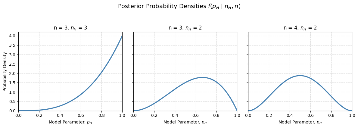
By stacking every possible outcome, \(n_H\), on the vertical axis of a colormap plot, the global behavior of the estimator is shown for different values of total tosses \(n\). For \(n=5\), the landscape is smeared and blurry; multiple values of \(p_H\) can reasonably explain the data. As \(n\) climbs to \(50\), the probability mass violently condenses along a sharp diagonal ridge where \(p_H \approx \frac{n_H}{n}\). In the limit of \(n \rightarrow + \infty\), the pdf behaves more and more like a Dirac’s delta in \(\frac{n_H}{n}\).
# --- FIGURE 2: Series of Colormaps for Different Values of n ---
n_values = [5, 20, 50]
p_H_mesh = np.linspace(0, 1, 200)

fig, axs = plt.subplots(1, len(n_values), figsize=(12, 4))
fig.suptitle("Posterior Density Map $f(p_H \\mid n_H, n)$ as Sample Size ($n$) Grows", fontsize=14, y=1.02)

for idx, n in enumerate(n_values):
    n_H_values = np.arange(0, n + 1)

    # Create a 2D grid of densities: rows = n_H, columns = p_H
    density_matrix = np.zeros((len(n_H_values), len(p_H_mesh)))

    for i, n_H in enumerate(n_H_values):
        # Compute the continuous analytical posterior density across the p_H line
        density_matrix[i, :] = beta.pdf(p_H_mesh, n_H + 1, n - n_H + 1)

    # Plot using pcolormesh to get a continuous distribution along the x-axis
    im = axs[idx].pcolormesh(p_H_mesh, n_H_values, density_matrix, shading='auto', cmap='viridis')

    axs[idx].set_title(f"Total Tosses, n = {n}", fontsize=12)
    axs[idx].set_xlabel("Model Parameter, $p_H$")
    axs[idx].set_ylabel("Number of Heads, $n_H$")

    # Add a colorbar for each plot to show density scale
    cbar = fig.colorbar(im, ax=axs[idx], orientation='vertical')
    cbar.ax.tick_params(labelsize=8)

plt.tight_layout()
plt.show()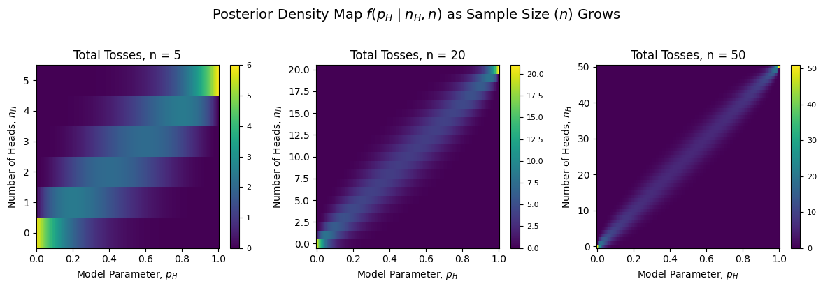
Stripping away the smooth gradients reveals the exact boundaries of our confidence. These pixelated bands show the \(95\%\) and \(99\%\) “Credible Intervals”. For a given experimental outcome \(n_H\), reading horizontally across the dark gray band gives the exact range of coin biases you should rationally accept.
Notice how the bands naturally pinch and become asymmetric near the physical boundaries (\(0.0\) and \(1.0\)), beautifully showcasing how Bayesian math inherently respects the physical limits of probability without any artificial mathematical fixes.
import numpy as np
import matplotlib.pyplot as plt
from scipy.stats import beta

# Define the sample sizes (n) for the subplots
n_values = [5, 20, 50]
p_H_mesh = np.linspace(0, 1, 500)

fig, axs = plt.subplots(1, len(n_values), figsize=(12, 4))
fig.suptitle("Bayesian Credible Intervals (95% and 99%) as Sample Size, $n$, Grows", fontsize=14, y=1.02)

for idx, n in enumerate(n_values):
    n_H_values = np.arange(0, n + 1)

    # Initialize a grid filled with 0 (White/Background)
    # Dimensions: rows = n_H, columns = p_H
    interval_matrix = np.zeros((len(n_H_values), len(p_H_mesh)))

    for i, n_H in enumerate(n_H_values):
        # Under a uniform prior, the posterior is Beta(n_H + 1, n - n_H + 1)
        posterior = beta(n_H + 1, n - n_H + 1)

        # Compute symmetric intervals
        # 95% Interval bounds (leaves 2.5% in each tail)
        lower_95 = posterior.ppf(0.025)
        upper_95 = posterior.ppf(0.975)

        # 99% Interval bounds (leaves 0.5% in each tail)
        lower_99 = posterior.ppf(0.005)
        upper_99 = posterior.ppf(0.995)

        # Fill the row based on threshold conditions:
        # Assign 1 for the 99% region (Light Gray)
        mask_99 = (p_H_mesh >= lower_99) & (p_H_mesh <= upper_99)
        interval_matrix[i, mask_99] = 1

        # Assign 2 for the 95% region (Darker Gray), overwriting the inner part
        mask_95 = (p_H_mesh >= lower_95) & (p_H_mesh <= upper_95)
        interval_matrix[i, mask_95] = 2

    # Map our integer codes (0, 1, 2) to specific grayscale values
    # 0 -> White, 1 -> Light Gray, 2 -> Darker Gray
    from matplotlib.colors import ListedColormap
    gray_cmap = ListedColormap(['#ffffff', '#d3d3d3', '#808080'])

    # Plot the matrix
    im = axs[idx].pcolormesh(p_H_mesh, n_H_values, interval_matrix,
                             shading='auto', cmap=gray_cmap, vmin=0, vmax=2)

    axs[idx].set_title(f"Total Tosses, n = {n}", fontsize=12)
    axs[idx].set_xlabel("Model Parameter, $p_H$")
    axs[idx].set_ylabel("Number of Heads, $n_H$")
    axs[idx].grid(True, linestyle=":", alpha=0.3, color='black')

# Add a custom legend to the last subplot to explain the discrete bands
from matplotlib.patches import Patch
legend_elements = [
    Patch(facecolor='#808080', edgecolor='none', label='95% Credible Interval'),
    Patch(facecolor='#d3d3d3', edgecolor='none', label='99% Credible Interval'),
    Patch(facecolor='#ffffff', edgecolor='gray', label='Outside Bounds')
]
axs[-1].legend(handles=legend_elements, loc='lower right', frameon=True)

plt.tight_layout()
plt.show()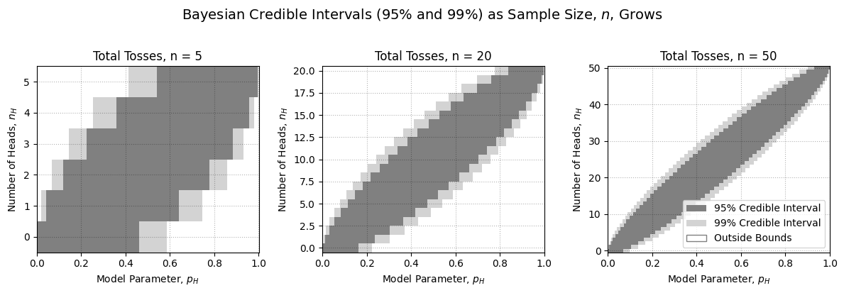
Discussion of the fair coin assumption, using Bayesian approach. The fair coin assumption can be stated as “\(p_H = 0.5\)”. Here two “credible intervals” are defined and shown. If the \(p_H\) value of the assumption lies outside a \(c\%\) credible interval, there’s only \(c\%\) of probability that the observed data are compatible with the assumption: discarting the assumption has only \(c\%\) of probability of being wrong.
At \(n = 5\), it’s possible to discard the “fair coin assumption” with a 5% error probability if the observed data contains \(n_H = 0\) (0%) Heads or \(n_H = 5\) (100%) Heads. With only 5 tosses, it is never possible to discard the assumption with a 1% error probability, as the 99% interval is wide enough to contain \(p_H = 0.5\) for all outcomes.
At \(n = 20\), the fair coin assumption can be discarded with a 5% error probability if \(n_H \le 5\) (\(\le 25\%\)) or \(n_H \ge 15\) (\(\ge 75\%\)). It can be discarded with a 1% error probability if the outcome is even more extreme: \(n_H \le 4\) (\(\le 20\%\)) or \(n_H \ge 16\) (\(\ge 80\%\)).
At \(n = 50\), the narrower credible intervals allow us to detect much smaller deviations. The fair coin assumption can now be discarded with a 5% error probability if \(n_H \le 17\) (\(\le 34\%\)) or \(n_H \ge 33\) (\(\ge 66\%\)). To achieve a strict 1% error probability, the required threshold shifts to \(n_H \le 14\) (\(\le 28\%\)) or \(n_H \ge 36\) (\(\ge 72\%\)).
Coin tosses as dependent events. Can multiple coin tosses be not independent? A first situation it comes into my mind is some accumulation of weight on the bottom side after a toss, as in the case the coin lands on a surface that could leave some material on the lower side. This condition unbalance the coin, moving the center of gravity of the coin towards the lower side of the first toss and making the outcome of the second toss be the same as the first one more likely.↩︎