Natural modes in structures

This post tries to answer a narrow question I’ve found on Physics SE, mainly about some doubts the OP¹ had about standing waves — or natural or proper modes of vibration —, their definition and the role of boundary conditions in the differential problem, and response to external forcing arising from the YouTube video, Standing Waves Parti I: Demonstration, by James Dann, Ph.D.

Natural modes

Many structural problems are governed by a differential problem, whose discret(ized) counterpart is a second order dynamical system,

\[\mathbf{M} \ddot{\mathbf{u}} + \mathbf{C} \dot{\mathbf{u}} + \mathbf{K} \mathbf{u} = \mathbf{f} \ ,\]

supplied with the proper conditions on the state \(\mathbf{u}(t)\), like initial values of the function and its first derivative for Cauchy problems (or initial value problems),

Remarks

• This is a linear problem, and its solution can be written as a linear combination of a set of solutions

• Proper modes: a basis for the non-trivial solution of the homogenous problem, i.e. the response of the system to a free system with no external forcing, to a non-zero initial condition

• Mass matrix \(\mathbf{M}\) and stiffness matrix \(\mathbf{K}\) are symmetric, if dynamical equations are derived with a Lagrangian approach. Here a proof for rigid-body mechanical systems.

• If no rigid degree of freedom exists, stiffness matrix is definite positive. If \(n_r\) independent degrees of freedom exists, stiffness matrix is semi-definite positive with a kernel of dimension \(n_r\) (or it’s \(n_r\) times singular).

• If there’s no degree of freedom associated with zero-inertia, mass matrix is definite positive. Independent d.o.f.s with zero-inertia are usually associated with algebraic constraints: if corresponding d.o.f.s are not expressed as a function of the other d.o.f.s, mass matrix is semi-definite positive (with kernel of dimension \(n_c\), whose elements are the mass-less d.o.f.s; or it’s \(n_c\) times singular), and the governing equations can be written as a system of DAEs (dynamical-algebraic equations).

• The modes of an undamped system, \(\mathbf{C} = \mathbf{0}\), simultaneously diagonalize mass and stiffness matrices. As a consequence of matrix symmetry, it’s easy to prove that modes are mutually orthogonal through mass and stiffness matrices

  \[\begin{aligned} \mathbf{u}_i^T \mathbf{M} \mathbf{u}_j & = m_i \delta_{ij} & \text{(no sum)} \\ \mathbf{u}_i^T \mathbf{K} \mathbf{u}_j & = k_i \delta_{ij} & \text{(no sum)} \\ \end{aligned}\]

• Mechanical systems with no dampers usually have small damping. This condition is treated in detail here. In the small-damping regime, damping matrix \(\mathbf{C}\) can be treated as a small perturbation of the undamped system, and two assumptions emerge as reasonable assumptions:

  • \(\mathbf{C}\) is semi-definite positive

  • modal basis \(\{ \hat{\mathbf{u}}_i \}\) makes the damping matrix \(\mathbf{C}\) diagonal

    \[\hat{\mathbf{u}}^T_i \mathbf{C} \hat{\mathbf{u}}_j = c_i \delta_{ij} \ ,\]

    as well.

• If many eigenvectors exist with the same eigenvalue, it’s possible to define an orthogonal basis of that subspace

• …

String

Governing equations

The transverse displacement \(u(x,t)\) of a string with axial (tension) pre-load \(N_0\) and linear mass density \(m\) is governed by the partial differential equation

\[- m \ddot{u} + N_0 u'' = f\]

supplied with proper boundary and initial conditions. Here \(f(x,t)\) is the transverse force per unit-length acting on the string.

Natural modes

Response to motion of an extreme point (as external forcing)

Exploiting the linearity of the problem, the solution can be written as the sum of a forced and an homogeneous part,

\[u(x,t) = u_0(x,t) + u_p(x,t) \ .\]

…some words about slow and fast contributions in structural mechanics, direct truncation and mode acceleration,…

Here \(f = 0\),

\[\begin{cases} - m \ddot{u} + N_0 u'' = 0 & , \quad \text{$(x,t) \in [0,b] \times [0, t_{max}]$} \\ u(0,t) = 0 & , \quad \text{$t \in [0,t_{max}]$} \\ u(b,t) = u_B(t) \\ u(x,0) = u_0(x) & , \quad \text{$x \in [0,b]$} \\ \dot{u}(x,0) = v_0(x) \end{cases}\]

Fast part

Fast part of the solution takes into account non-homogeneous boundary conditions and other external forces. It can be defined through its governing equation

\[\begin{cases} N_0 u''_p = 0 & , \quad \text{$(x,t) \in [0,b] \times [0, t_{max}]$} \\ u_p(0,t) = 0 & , \quad \text{$t \in [0,t_{max}]$} \\ u_p(b,t) = u_B(t) \\ \end{cases}\]

whose solution reads

\[u_p(x,t) = u_B(t) \frac{x}{b} \ .\]

Slow part

Slow part takes into account the remaining part of the problem

\[\begin{cases} - m \ddot{u}_0 + N_0 u''_0 = m \ddot{u}_p - N_0 \underbrace{u''_p}_{=0} & , \quad \text{$(x,t) \in [0,b] \times [0, t_{max}]$} \\ u_0(0,t) = 0 & , \quad \text{$t \in [0,t_{max}]$} \\ u_0(b,t) = 0 \\ u_0(x,0) = u(x,0) - u_p(x,0) & , \quad \text{$x \in [0,b]$} \\ \dot{u}_0(x,0) = \dot{u}(x,0) - \dot{u}_p(x,0) \end{cases}\]

The solution of this problem can be written as a linear combination

\[u_0(x,t) = \sum_n g_n(t) \, f_n(x) \ ,\]

of the proper modes,

\[f_n(x) = \sin \left( k_n x \right) \ ,\]

with \(k_n = \frac{n \pi}{b}\), whose time-dependent amplitudes read

\[g_n(t) = a_n \cos \left( \omega_n t \right) + b_n \sin \left( \omega_n t \right) \ ,\]

with \(\omega_n = c k_n = \sqrt{\frac{N_0}{m}} \frac{n \pi}{b}\), and coefficients \(a_n\), \(b_n\) evaluated to match the initial conditions.

Solution

Exploiting orthogonality of harmonic functions,

\[\begin{aligned} \int_{0}^{b} \sin \left(\frac{n \pi x}{b}\right) \sin \left(\frac{m \pi x}{b} \right) \, dx & = \frac{b}{2} \delta_{nm} \\ \int_{0}^{b} \cos \left(\frac{n \pi x}{b}\right) \cos \left(\frac{m \pi x}{b} \right) \, dx & = \frac{b}{2} \delta_{nm} \\ \int_{0}^{b} \sin \left(\frac{n \pi x}{b}\right) \cos \left(\frac{m \pi x}{b} \right) \, dx & = 0 \\ \end{aligned}\]

and projection of the solution onto these functions,

\[\begin{aligned} 0 & = \int_{x=0}^{b} \sin\left( \dfrac{m \pi x}{b} \right) \left\{ - m \ddot{u}_0 + N_0 u''_0 - m \ddot{u}_p \right\} dx = \\ & = \int_{x=0}^{b} \sin\left( \dfrac{m \pi x}{b} \right) \sum_n \left\{ - m \ddot{g}_n(t) - k^2_n N_0 g_n(t) \right\} \sin \left( \dfrac{n \pi x}{b} \right) \, dx - \int_{x=0}^b \sin\left( \dfrac{m \pi x}{b} \right) m \frac{x}{b} dx \, \ddot{u}_B(t) \end{aligned}\]

the PDEs can be recast as a (infinite dimension) linear system

\[m \dfrac{b}{2} \ddot{g}_n(t) + k^2_n N_0 \dfrac{b}{2} g_n(t) = (-1)^{n} m \dfrac{b}{\pi n} \ddot{u}_B(t) \ , \]

or, dividing by the mass \(m\) times \(\frac{b}{2}\) and recalling that \(k_n = \frac{n \pi}{b}\), \(c := \sqrt{\frac{N_0}{m}}\) and \(\omega_n := c k_n\),

\[\ddot{g}_n(t) + \omega_n^2 g_n(t) = (-1)^{n} \dfrac{2}{\pi n} \ddot{u}_P(t) \ ,\]

being

\[\begin{aligned} \int_{x=0}^b \dfrac{x}{b} \sin \left( \dfrac{m \pi x}{b} \right) dx & = \left.\left[ - \dfrac{x}{b} \dfrac{b}{\pi m} \cos\left( \dfrac{m \pi x}{b} \right) \right]\right|_{x=0}^{b} + \int_{x=0}^{b} \dfrac{1}{\pi m} \cos \left( \dfrac{m \pi x}{b} \right) \, dx = \\ & = - \dfrac{b}{\pi m} \underbrace{\cos\left( m \pi \right)}_{(-1)^m} + \underbrace{\dfrac{b}{(\pi m)^2} \left.\sin\left( \dfrac{m \pi x}{b} \right)\right|_{x=0}^{b}}_{=0} = \\ & = -(-1)^{m} \dfrac{b}{\pi m} \ . \end{aligned}\]

The solution of the equation for \(g_n\) can be written as the sum of the solution of the homogeneous equation and an independent particular solution \(g_{n,P}\)

\[g_n(t) = a_n \cos \left( \omega_n t \right) + b_n \sin \left( \omega_n t \right) + g_{n,P}(t) \ .\]

Sligthly damped system

Mechanical systems without any damper element usually have small damping, that can be well represented as a modal damping. Under this assumption, the modal equations become

\[\ddot{g}_n(t) + 2 \xi_n \omega_n \dot{g}_n(t) + \omega_n^2 g_n(t) = (-1)^{n} \dfrac{2}{\pi n} \ddot{u}_B(t) \ ,\]

with \(\xi_n \ll 1\). The eigenvalues of the equation comes from the solution of the algebraic equation

\[s^2 + 2 \xi_n \omega_n s + \omega^2_n = 0 \qquad \rightarrow \qquad s_{1,2} = - \xi_{n} \omega_n \mp \sqrt{\xi_n^2 \omega_n^2 - \omega^2_n} = \omega_n \left[ -\xi_n \mp i \sqrt{ 1 - \xi_n^2 } \right] \ ,\]

and the solution of the homogeneous equation reads

\[\begin{aligned} g_{n,0}(t) & = c_n e^{\left(- \xi_n \mp i \sqrt{1-\xi^2_n} \right) \omega_n t} + \text{ c.c.} = \\ & = a_n e^{-\xi_n \omega_n t} \cos\left( \sqrt{1 - \xi^2_n} \, \omega_n t \right) + b_n e^{-\xi_n \omega_n t} \sin\left( \sqrt{1 - \xi^2_n} \, \omega_n t \right) \end{aligned}\]

If the damping is non-zero, \(\xi_n > 0\), and the homogeneous part of the solution \(g_{n,0}(t)\) goes to zero for sufficient long time,

\[\lim_{t \rightarrow + \infty} g_{n,0}(t) \rightarrow 0 \ ,\]

and thus the free response of the system — and the effect of the initial condition — becomes negligible and only the forced response is relevant.

Harmonic forcing

With \(u_B(t) = U \sin \left( \Omega t \right)\), the particular solution has the expression

\[g_{n,P}(t) = A_n \cos\left( \Omega t \right) + B_n \sin\left( \Omega t \right) \ , \]

whose coefficients \(A_n\), \(B_n\) can be evaluated matching harmonic terms

\[ \begin{bmatrix} -\Omega^2+\omega_n^2 & 2 \xi_n \omega_n \Omega \\ -2 \xi_n \omega_n \Omega & -\Omega^2+\omega_n^2 \end{bmatrix} \begin{bmatrix} A_n \\ B_n \end{bmatrix} = \begin{bmatrix} 0 \\ 1 \end{bmatrix} (-1)^{n+1} \dfrac{2}{\pi n} U \Omega^2 \]

\[\begin{aligned} \begin{bmatrix} A_n \\ B_n \end{bmatrix} & = \dfrac{1}{\left( - \Omega^2 + \omega^2_n \right)^2 + \left( 2 \xi_n \omega_n \Omega \right)^2} \begin{bmatrix} -\Omega^2+\omega_n^2 & -2 \xi_n \omega_n \Omega \\ 2 \xi_n \omega_n \Omega & -\Omega^2+\omega_n^2 \end{bmatrix} \begin{bmatrix} 0 \\ 1 \end{bmatrix} (-1)^{n+1} \dfrac{2}{\pi n} U \Omega^2 = \\ & = (-1)^{n+1} \dfrac{2}{\pi n} \dfrac{\Omega^2}{\left(-\Omega^2 + \omega^2_n \right)^2 + \left( 2 \xi_n \omega_n \Omega \right)^2} \begin{bmatrix} -2 \xi_n \omega_n \Omega \\ -\Omega^2 + \omega^2_n \end{bmatrix} U \ . \end{aligned}\]

Exploiting properties of harmonic functions, the particular solution can be recast as

\[\begin{aligned} \dfrac{g_{n,P}(t)}{U} & = A_n \cos(\Omega t ) + B_n \sin(\Omega t ) = \\ & = C_n \sin(\Omega t + \varphi_n ) = \\ & = C_n \left( \dfrac{A_n}{C_n} \cos(\Omega t) + \dfrac{B_n}{C_n} \sin(\Omega t) \right) = \\ & = C_n \left( \sin \varphi_n \cos(\Omega t) + \cos \varphi_n \sin(\Omega t) \right) \ , \end{aligned}\]

with gain \(C_n = \sqrt{A^2_n + B^2_n}\), i.e.

\[\begin{aligned} C_n & = \dfrac{2}{\pi n} \dfrac{\Omega^2}{\left(-\Omega^2 + \omega^2_n \right)^2 + \left( 2 \xi_n \omega_n \Omega \right)^2}\sqrt{\left(-\Omega^2 + \omega^2_n \right)^2 + \left( 2 \xi_n \omega_n \Omega \right)^2} = \\ & = \dfrac{2}{\pi n} \dfrac{\Omega^2}{\sqrt{\left(-\Omega^2 + \omega^2_n \right)^2 + \left( 2 \xi_n \omega_n \Omega \right)^2}} = \\ & = \dfrac{2}{\pi n} \dfrac{\left(\frac{\Omega}{\omega_n}\right)^2}{\sqrt{\left(1 - \left(\frac{\Omega}{\omega_n}\right)^2 \right)^2 + \left( 2 \xi_n \frac{\Omega}{\omega_n} \right)^2}} \ , \end{aligned}\]

and phase delay \(\varphi_n\) s.t.

\[ \varphi_n = \text{atan2}\left( a \sin \varphi_n, a \cos \varphi_n \right) = \text{atan2}\left( A_n, B_n \right) = \left( (-1)^{n} \cdot 2 \xi_n \omega_n \Omega , (-1)^{n} ( \Omega^2 - \omega_n^2 ) \right) \ ,\]

having exploited the definition of an \(\text{atan2}(\cdot)\) function, whose co-domain width is \(2\pi\).

Gain as a function of frequency \(\Omega\) of the forcing.

\[f(x) = \dfrac{x^2}{\left( ( 1 - x^2)^2 + 4 \xi^2 x^2 \right)^{\frac{1}{2}}}\]

\[\begin{aligned} f'(x) & = \dfrac{2 x ( ( 1 - x^2)^2 + 4 \xi^2 x^2 )^{\frac{1}{2}} - x^2 \frac{1}{2} ( ( 1 - x^2)^2 + 4 \xi^2 x^2 )^{-\frac{1}{2}} \left( - 2 ( 1 - x^2 ) \cdot 2 x + 8 \xi^2 x \right) }{(1-x^2)^2 + 4 \xi^2 x^2} = \\ & = \dfrac{ 2x - 4 x^3 + 2 x^5 + 8 \xi^2 x^3 - \left( - 2 x^3 + 2 x^5 + 4 \xi^2 x^3 \right) }{\left\{(1-x^2)^2 + 4 \xi^2 x^2\right\}^{\frac{3}{2}}} = \\ & = \dfrac{ 2x - 2 x^3 + 4 \xi^2 x^3}{\left\{(1-x^2)^2 + 4 \xi^2 x^2\right\}^{\frac{3}{2}}} = \\ & = \dfrac{ 2 x ( 1 - ( 1 - 2 \xi^2 ) x^2)}{\left\{(1-x^2)^2 + 4 \xi^2 x^2\right\}^{\frac{3}{2}}} = \\ \end{aligned}\]

a maximum exists for \(\bar{x} = \frac{1}{\sqrt{1- 2 \xi^2}}\), if \(\xi < \frac{1}{\sqrt{2}}\),

\[\begin{aligned} f(\bar{x}) & = \dfrac{\frac{1}{1-2\xi^2}}{\left( \left( 1 - \frac{1}{1-2\xi^2} \right)^2 + 4 \xi^2 \frac{1}{1 - 2 \xi^2}\right)^{\frac{1}{2}}} = \\ & = \dfrac{1}{\left( 4 \xi^4 + 4 \xi^2 ( 1- 2 \xi^2) \right)^{\frac{1}{2}}} = \\ & = \frac{1}{2 \xi (1-\xi^2)^{\frac{1}{2}}} \end{aligned}\]

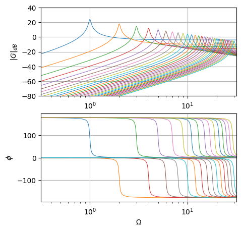
#> Some libraries
import numpy as np
from scipy import signal
import matplotlib.pyplot as plt

#> Bode diagram of the natural modes

#> Parameters of the system (non-dimensional)
m, N0, b = 1., 1., np.pi
c = np.sqrt(N0/m)
xi = .02

n_modes = 30
i_modes = np.arange(1, n_modes+1)
omegas = 10.**np.linspace(-.5, 1.5, 1000)

fig, ax = plt.subplots(2,1, figsize=(5, 5))

for i_mode in i_modes:
    #> Mode parameters
    k_n = i_mode * np.pi / b
    omega_n = k_n * c
    xi_n = xi

    #> Continuous-time TF (no dt is given as a third argument in signal.TransferFunction)
    # defined with numerator and denominator
    num = np.array([1, 0, 0]) * (-1)**(i_mode+1) * 2. / ( np.pi * i_mode )
    den = np.array([1, 2*xi_n*omega_n, omega_n**2])
    sys = signal.TransferFunction(num, den)

    #> Evaluation of magnitude and phase of the TF of the LTI system sys
    # mag is in dB i.e. |G|_{dB} = 20 log_10{|G|}se
    w, mag, phase = signal.bode(sys, omegas)

    #> Plot
    ax[0].semilogx(omegas, mag  , lw=.7)
    ax[1].semilogx(omegas, phase, lw=.7)

G_ticks = 20 * np.arange(-4,3)
ax[0].set_yticks(G_ticks)
ax[0].set_xlim(omegas[0], omegas[-1]);  ax[0].grid()
ax[0].set_ylim(G_ticks[0], G_ticks[-1])
ax[1].set_xlim(omegas[0], omegas[-1]);  ax[1].grid()
ax[0].set_ylabel('$|G|_{dB}$')
ax[1].set_xlabel('$\Omega$')
ax[1].set_ylabel('$\phi$')

Text(0, 0.5, '$\\phi$')

Full solution

Full solution of the problem with the prescribed motion \(u_B(t) = U \sin(\Omega t)\) reads

\[\begin{aligned} u(x,t) & = \left\{ \frac{x}{b} \sin(\Omega t) + \sum_n \sin \left( k_n x \right) g_{n,p}(t) \right\} U_B + \sum_{n} C_{n,0} \sin( k_n x ) e^{-\xi_n \omega_n t} \cos \left( \sqrt{1 - \xi^2_n} \, \omega_n t - \varphi_{n,0} \right) \\ & = \left\{ \frac{x}{b} \sin(\Omega t) + \sum_n \sin \left( k_n x \right) C_n(\Omega) \sin(\Omega t + \varphi_n(\Omega) ) \right\} U_B + \sum_{n} C_{n,0} \sin( k_n x ) e^{-\xi_n \omega_n t} \cos \left( \sqrt{1 - \xi^2_n} \, \omega_n t + \varphi_{n,0} \right) \end{aligned}\]

s.t. its time derivative \(\partial_t u(x,t)\) is

\[\begin{aligned} \dot{u}(x,t) & = \left\{ \frac{x}{b} \cos(\Omega t) + \sum_n \sin \left( k_n x \right) C_n(\Omega) \cos(\Omega t + \phi_n(\Omega) ) \right\} \Omega U_B + \sum_{n} C_{n,0} \sin( k_n x ) e^{-\xi_n \omega_n t} \left[ - \xi_n \omega_n \cos \left( \sqrt{1 - \xi^2_n} \, \omega_n t + \varphi_{n,0} \right) - \sqrt{1-\xi_n^2} \omega_n \sin\left( \sqrt{1 - \xi^2_n} \, \omega_n t + \varphi_{n,0} \right) \right] \end{aligned}\]

Both forced and free response can be re-written as the sum of a \(\sin\) and \(\cos\) contribution per each wave number. The coefficients \(A_n\), \(B_n\) of the forced response have already been evaluated above. The coefficients of the free response \(A_{0,n}\), \(B_{0,n}\) need to be evaluated with the initial conditions.

\[f(t) = e^{-\xi \omega t} \left[ A_0 \cos(\widetilde{\omega} t) + B_0 \sin(\widetilde{\omega} t) \right]\]

\[\dot{f}(t) = e^{-\xi \omega t} \left[ A_0 \left( -\xi \omega \cos(\widetilde{\omega} t) - \widetilde{\omega} \sin(\widetilde{\omega} t) \right) + B_0 \left(-\xi \omega \sin(\widetilde{\omega} t) + \widetilde{\omega} \cos(\widetilde{\omega} t) \right) \right]\]

Solving for initial conditions

Projection to find a linear system for the coefficients \(A_{n,0}\), \(B_{n,0}\)…

\[u_0(x) = u(x,0) = \sum_{n} \sin(k_n x) A_n U_B + \sum_{n} A_{n,0} \sin(k_n x)\]

\[v_0(x) = \dot{u}(x,0) = \dfrac{x}{b}\Omega U_B + \sum_{n} B_n \Omega U_B \sin(k_n x) + \sum_{n} \left\{ - A_{n,0} \xi_n \omega_n + B_{n,0} \omega_n \sqrt{1 - \xi_n^2} \right\} \sin(k_n x)\]

This is a system of two equations, with infinite unknowns \(A_{n,0}\), \(B_{n,0}\). While this sounds like a very under-determined system, this is not the case since the two equations depends on the continuous spatial coordinate \(x\) and thus they’re 2 infinite-dimensional equations: each equation is not just an equality, but it’s an equality that needs to hold for every possible \(x \in [0,b]\), and thus each equation prescribes infinite constraints.

Now, infinite constraints and infinite unknowns…the problem looks trickier and trickier. But it’s quite easy to solve through projection on the functions \(\sin( k_p x )\) exploiting the orthogonality of these harmonic functions on the interval \([0,b]\). This process should recall to the reader the Fourier series expansion of periodic functions. The equations become an infinite number of decoupled pairs of equations,

\[\int_{x=0}^{b} \sin(k_p x) u_0(x) dx = \dfrac{b}{2} \left( A_p U_B + A_{p,0} \right)\]

\[\int_{x=0}^{b} \sin(k_p x) \left( v_0(x) - \dfrac{x}{b} \Omega U_B \right) \, dx = \dfrac{b}{2} \left( B_p \Omega U_B + \omega_p \left( - \xi_p A_{p,0} + \sqrt{1 - \xi^2_p} B_{p,0} \right) \right)\]

whose results are easily evaluated as

\[\begin{aligned} A_{p,0} & = - A_p U_B + \dfrac{2}{b} \int_{x=0}^{b} \sin(k_p x) u_0(x) \, dx \\ B_{p,0} & = \dots \end{aligned}\]

Footnotes

1. Slang proper of Stack Exchange and other forums, OP means Original Poster.